Introduction to Quantum Computing with IBM Hardware - Quantum Computing & Quantum Information

Quantum Computing is developing into one of the promising approaches to solve questions that classical conventional computers cannot easily handle or intractable at all. Using its power of entanglement and superposition, which will be covered later, that quantum systems possess, quantum algorithms have the potential to provide sped-up (exponential or quadratic)computation over classical algorithms. Quantum computers and computing has developed a lot over the past few years, and although they have not yet been identified as universal quantum computers, their development has shown advantages over conventional computers. Using the IBM Quantum Platform, we are able to implement and run certain algorithms with limited number of qubits.

Background¶

This section is meant to introduce some of the basic ideas and and concepts from quantum mechanics and then get into quantum computing!

1 Quantum Concepts¶

1.1 Qubit¶

In general, any two-level quantum system can be treated as qubit, which can be in either quantum state of $|0\rangle$ and $|1\rangle$ . Similar to classical bits (eg. on/off, high voltage/low voltage as 0/1), there are lots of systems that can realize such quantum systems such as the spin of atoms or electrons (up/down), or the occupation number of fermions in optical lattices (0/1). Quantum computing methods have pointed into different directions like trapped-ion, electron on helium, optical lattices, and photonic.

We mentioned the states $|0\rangle$ and $|1\rangle$ as :

| 0 \rangle = \begin{pmatrix} 1 \\ 0 \end{pmatrix} \qquad |1 \rangle = \begin{pmatrix} 0 \\ 1 \end{pmatrix}

(1)

$| \psi \rangle$ is called a “ket” and $\langle \phi |$ is called a “bra”. They are related through $\langle i | = | i \rangle^\dagger$ . These states form an orthonormal basis of the Hilbert space $\langle i | j \rangle = \delta_{i,j}$ . These are all part of the Dirac Notation, which you can learn more about in Chapter 1.

1.2 Pauli Matrices¶

The Pauli matrices, defined as below, is a set of unitary ( $U U^\dagger = U^\dagger U = \mathcal{I}$ ) and Hermitian ( $U^\dagger = U$ ) $2\times2$ complex matrices.

\sigma_x = \begin{pmatrix} 0 & 1 \\1 & 0 \end{pmatrix} \qquad \sigma_y = \begin{pmatrix} 0 & -i \\i & 0 \end{pmatrix} \qquad\sigma_z = \begin{pmatrix} 1 & 0 \\0 & -1 \end{pmatrix}

(2)

1.3 Superposition of quantum states¶

One quantum state can be written as the superposition of other quantum states with complex coefficients. The interpretation is to represent this state in another orthonormal space.

|\psi\rangle = \sum_i \alpha_i |\phi_i \rangle

(3)

Another important set of states to know is the superposition of $| 0 \rangle$ and $| 1 \rangle$ , shown as

| + \rangle = \frac{1}{\sqrt{2}} \left( |0\rangle + |1\rangle \right) \qquad | - \rangle = \frac{1}{\sqrt{2}} \left( |0\rangle - |1\rangle \right)

(4)

which are eigenstates of Pauli-X matrix.

1.4 Bloch Sphere¶

The bloch sphere is one way to visualize the state of one qubit. A general state of one qubit can be written as,

| \psi \rangle = \cos(\theta/2) | 0 \rangle + \sin(\theta/2) e^{i \phi} | 1 \rangle

(5)

from IPython.display import Image
Image ("blochsphere.png", width=500)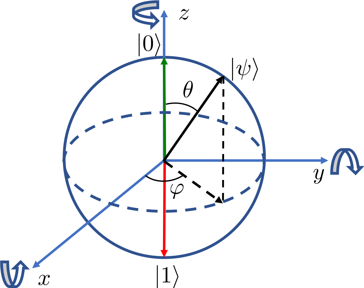

where the $| + \rangle$ and $|- \rangle$ states sit on the X-axis. Chapter 2 looks a little deeper into qubits, states, and the bloch sphere.

1.5 Entanglement¶

Entanglement is a quantum feature of a system of multiple qubits. A entangled state cannot be separated, which means the system cannot be expressed as two independent subsystem.

| \psi \rangle \neq | \psi_A \rangle \otimes | \psi_B \rangle

(6)

One example of entangled states is a Bell state:

| \psi \rangle = \frac{1}{\sqrt{2}} \Big( | 0_A 0_B \rangle + | 1_A 1_B \rangle \Big)

(7)

1.5.1 Density operator and von Neumann entropy¶

The density operator is useful to describe a statistical system in general. It has the definition as

\rho = \sum_i^n p_i | \psi_i \rangle \langle \psi_i |

(8)

where $n \ge 1$ , and $p_i$ is the probability of being in the state of $| \psi_i \rangle$ . When $n=1$ , the system is consider a pure state, or a mixed state otherwise. The trace of a density matrix is always one $tr(\rho)=1$ , and a pure state also satisfies the condition that $\rho = \rho^2$ .

The von Neumann entropy is defined as,

S_{vN}(\rho) = - tr(\rho \ln \rho)

(9)

and it is easy to prove that the entropy of a pure state is zero.

The entropy of a subsystem is also related to measure entanglement to the rest of the system. To obtain the density matrix of a subsystem, we can “trace over” the rest of the system (sometime called environment). Consider a system $\rho$ , consists two subsystem A and B.

\begin{align} \rho_A &= tr_B (\rho) \\ &= \sum_j^{dim(B)} \langle \phi_j | \rho | \phi_j \rangle \end{align}

(10)

HW: Prove a non-entangled state, in the form of $| \psi \rangle = | \psi_A \rangle \otimes | \psi_B \rangle$ , has a density operator of the subsystem A as $\rho_A = | \psi_A \rangle \langle \psi_A |$ , and the entropy is zero.

For an entangled state like a Bell state, $| \psi \rangle = \frac{1}{\sqrt{2}} \Big( | 0_A 0_B \rangle + | 1_A 1_B \rangle \Big)$ , the density operator of system is:

\begin{align} \rho &= | \psi \rangle \langle \psi | \\ &= \frac{1}{2} \left( | 0_A 0_B \rangle \langle 0_A 0_B| +| 0_A 0_B \rangle \langle 1_A 1_B| +| 1_A 1_B \rangle \langle 0_A 0_B| +| 1_A 1_B \rangle \langle 1_A 1_B| \right) \\ \rho_A &= \langle 0_B | \rho | 0_B \rangle + \langle 1_B | \rho | 1_B \rangle \\ &= \frac{1}{2} \left( | 0_A \rangle \langle 0_A | + | 1_A \rangle \langle 1_A | \right) \end{align}

(11)

thus, the von Neumann entropy is $S_{vN}(\rho_A) = - 1/2 \ln (1/2) - 1/2 \ln (1/2) = ln 2$ . Learn about entangled states vs. product states and more in Chapter 3.

1.6 Quantum Gates¶

1.6.1 Single-qubit gates¶

A unitary matrix acts on one qubit is called single-qubit operation, or single-qubit gate. It is considered a rotation of a vector on Bloch sphere, transfer the state vector to a new position. For example, the Hadamard gate, expressed as below, transfer between $| 0 \rangle \leftrightarrow | + \rangle$ , and $| 1 \rangle \leftrightarrow | - \rangle$

H = \frac{1}{\sqrt{2}}\begin{pmatrix} 1 & 1 \\ 1 & -1 \end{pmatrix}

(12)

which can be consider as a rotation with respect to $45^\circ$ axis on X-Z plane.

Applying a gate that is unitary and Hermitian twice in a row will always gives you the identity matrix, and this feature can be used to simplify the circuit to prevent error of implementation.

1.6.2 Two-qubit gates¶

The operation acts on two qubits are always commonly used in quantum circuits. Utilizing two-qubit gates and single-qubit gates, an arbitrary quantum operation on multiple qubits can be approximated to an arbitrary accuracy, and those sets of gates are considered universal. One type of two-qubit gates plays an important role, controlled gate. A controlled gate, using one qubit as the control qubit and determine an operation on the target state. The operation will apply to the target state only if the control qubit is in $|1\rangle$

{}^{c}U|0a\rangle = |0a\rangle \qquad {}^{c}U|1a\rangle = |1\rangle U|a\rangle

(13)

I will introduce one important two-qubit gate, controlled-Not gate (CNOT).

\rm{CNOT} | 0 a \rangle = | 0 a \rangle \qquad \rm{CNOT} | 1 a \rangle = | 1 \bar{a} \rangle

(14)

HW: Try to prepare a Bell state mentioned above on two qubit, using CNOT. What about a quantum operation that swap the state of two qubit?

1.7 Quantum Circuits¶

Quantum circuits represent a set of sequential quantum gates on qubits to perform quantum computation. These quantum circuits are the fundamental unit of qiskit. A normal workflow of these circuits consist of building and then executing.

1.7.1 Building a Circuit¶

First we need to start with what we want to do, and in this case we are going to make a 3-qubit GHZ state system. We can do this by applying **gates** to the qubits. Let's look at how a we'd do this

|\psi\rangle = \left(|000\rangle+|111\rangle\right)/\sqrt{2}.

(15)

To create this state, we start with a 3-qubit register where each qubit is in a state of $|0\rangle$ by default. We then apply these gates:

A Hadamard gate ( $H$ ) on qubit 0, placing it into superposition state ( $|0\rangle + |1\rangle)/\sqrt(2)$
A Controlled-Not Gate ( $C_x$ or $CNOT$ ) between qubit 0 and 1.
A Controlled-Not Gate ( $C_x$ or $CNOT$ ) between qubit 0 and 2.
On a perfect no-noise quantum computer, these gates will apply a GHZ state. To do this in qiskit, we can write the the following:

from qiskit import QuantumCircuit #import qiskit and get QuantumCircuit to build our circuit

qc = QuantumCircuit(3) # name it qc (Quantum Circuit) and we want 3 qubits
#if we want classical bits, we'd do (3,2) for 2 classical bits as well 
qc.h(0) # apply Hadamard Gate to qubit 0
qc.cx(0,1) # apply our CNOT gate to qubit 0 and 1 
qc.cx(0,2) # apply another CNOT to qubit 0 and 2

<qiskit.circuit.instructionset.InstructionSet at 0x2b465dfb3d0>

With our circuit built, lets see what it looks like:

qc.draw('mpl') #the .draw('mpl') method with mpl(matplotlib)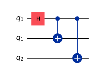

<Figure size 371.107x284.278 with 1 Axes>

In this circuit, we can see that our qubits and gates are applied as mentioned, a $Hadamard$ gate and 2 $CNOT$ gates, one to qubits (0,1) and another to (2,0). Below is an example of a circuit with more ‘depth’, or length.

Image("ibm_qAdder.png")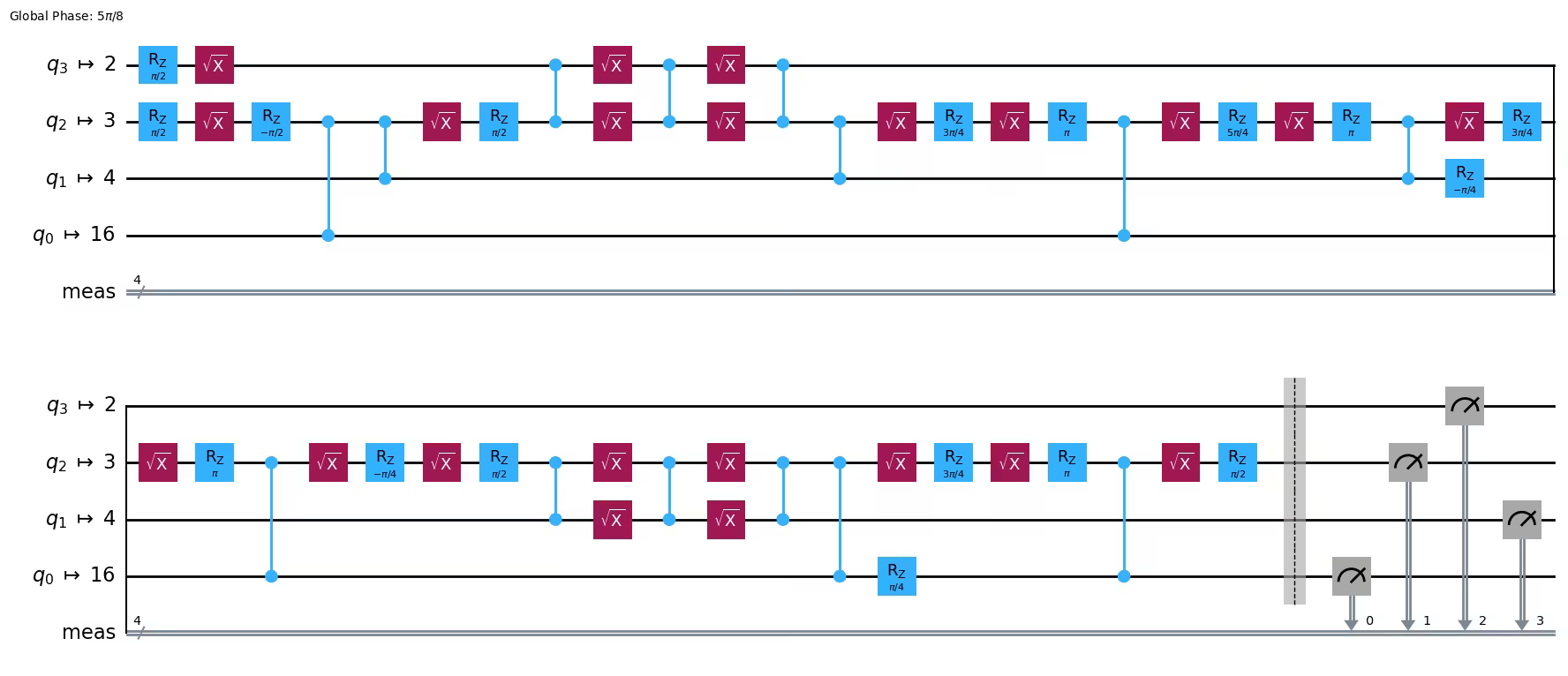

Here is an example of a transpiled quantum half-adder from IBM Quantum Platform Modules. For a broader overview of Quantum Circuits & Gates, take a look at Chapter 4 Summary.

1.8 IBM Quantum Platform and Experience¶

IBM Quantum Platform is a publically available resource where people can learn quantum computing, but it is also the home of their Quantum Composer where you can build quantum circuits like legos and run them on their hardware, which is what we’ll be doing. IBM also has their Introduction to Qiskit and IBM Quantum, where they teach you how to use their hardware and software. By using Qiskit, people have access to either their 156 or 127 qubit computers.

1.8.1 IBM Composer¶

IBM Composer is IBM’s visual ‘hands-on’ circuit builder. In their UI, you can see 5 different sections:

Gates : From Hadamard Gates to RC3X gates, you have multiple options on how you want to build your circuit
Circuit Editor : Here you actually build the circuit by adding gates, qubits, classical bits
Probability/Visualization : This section characterizes you circuit, or predicts what the outcome could be
Q-Sphere : This section visualizes your circuit on Bloch’s Sphere
Code : All aspects of your code are converted into code, either in OpenQASM or Qiskit
This interactive site allows people to build circuits and see whats happening in your circuit and what could happen.

1.8.2 Operations and Gates in IBM Composer¶

IBM Composer has many gates and operations from single-qubit, multi-qubit, and non-unitary operations. You can see the full list and what they do here. We’ll be looking at for 2 right now, which are the ones we used earlier, the Hadamard Gate and CNOT gate. Note that we want to see what happens to a qubit when we apply these gates, so we’ll be using qiskitAer, a circuit simulator from qiskit.

Hadamard Gate

H = \frac{1}{\sqrt{2}} \begin{pmatrix} 1 & 1\\ 1 & -1 \end{pmatrix}= u2(0,\pi)

(16)

from qiskit.quantum_info import Operator 
circuit = QuantumCircuit(2) # creating a new circuit here but still with qiskit
circuit.h(0)
circuit.draw('mpl') # draw our circuit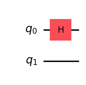

<Figure size 203.683x200.667 with 1 Axes>

op = Operator(circuit)
print(op.data.round(3))

[[1.+0.j 0.+0.j 0.+0.j 0.+0.j]
 [0.+0.j 0.+0.j 0.+0.j 1.+0.j]
 [0.+0.j 0.+0.j 1.+0.j 0.+0.j]
 [0.+0.j 1.+0.j 0.+0.j 0.+0.j]]

The 0.707 comes from the approximate value of $1/\sqrt(2)$ , meaning our gates were applied.

Cotrolled-Not Gate

The CNOT gate flips the target qubit when then control qubit is in the state $|1\rangle$ . Take the most significant bit as the control qubit and you get a matrix like :

C_X = \begin{pmatrix} 1 & 0 & 0 & 0\\ 0 & 1 & 0 & 0\\ 0 & 0 & 0 & 1\\ 0 & 0 & 1 & 0 \end{pmatrix}.

(17)

If you take the least significant bit and make it the control bit, then your matrix turns into :

C_X = \begin{pmatrix} 1 & 0 & 0 & 0\\ 0 & 0 & 0 & 1\\ 0 & 0 & 1 & 0\\ 0 & 1 & 0 & 0 \end{pmatrix}.

(18)

circuit.clear() #clear our circuit 
circuit.cx(0,1) # apply our CNOT gate to both qubits 
circuit.draw('mpl')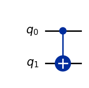

op = Operator(circuit)
print(op)

Operator([[1.+0.j, 0.+0.j, 0.+0.j, 0.+0.j],
          [0.+0.j, 0.+0.j, 0.+0.j, 1.+0.j],
          [0.+0.j, 0.+0.j, 1.+0.j, 0.+0.j],
          [0.+0.j, 1.+0.j, 0.+0.j, 0.+0.j]],
         input_dims=(2, 2), output_dims=(2, 2))

The output here shows our possible outcomes. Since we have 2 qubits, $2^2 = 4$ . 4 different possible states; $|00\rangle, |01\rangle, |10\rangle, |11\rangle$ .

2 Designing a quantum circuit¶

Designing a quantum circuit is a hard problem for a large system or complex problems. One way to realize simple algorithm is to study the decomposition of the target unitary matrix. When the system size is small, i.e. the dimension of the target unitary matrix is small, it is possible to decompose the matrix. In some other situations, the process of quantum algorithm can be implemented in the sequence of applying quantum gates on subsystems.

2.1 Quantum half-adder algorithm¶

Mentioned above, the quantum half-adder is a good example to start with due to its complexity. The input/output chart of such an adder can be expressed as:

Input bit 1	Input bit 2	Output bit 1	Output bit 2
0	0	0	0
0	1	0	1
1	0	0	1
1	1	1	0

The output bit 1 only flip from 0 to 1 when input bit 1 and input bit 2 are both 1. For the rest situation, it remains 0.
The output bit 2 is same as input bit 2 if input bit 1 is 0, and flips if input bit 1 is 1.

From these two rules, we are able to design a circuit.

The output bit 1 can be represented as the target qubit with a controlled-controlled-not gate with input bit 1 and input bit 2 are the control qubit.
The output bit 2 can be represented as the AND gate from input bit 1 and input bit 2, realized by a controlled-not gate. The circuit is then:

Image("quantum_half_adder.png")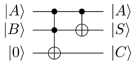

Next is to build circuit using the gates that IBM Qiskit provides. We can simplify the circuit from earlier by using a Toffoli gate, which is a CCX (Controlled-Controlled-NOT) gate. To create this circuit, we can start with out first slot (or step), which is to introduce our qubits and classical bits. 4 qubits, 2 qubits as out inputs, 1 to hold the ‘carry’ result, and 1 to hold the ‘sum’ result. Next, we prepare our 2 qubits, which in out case is $q_0$ and $q_1$ , where we can apply a ‘X-gate’ or Pauli-X gate to our qubits to change them from $| 0 \rangle$ into $|1 \rangle$ .

Image("OG_qAdder_circuit.png")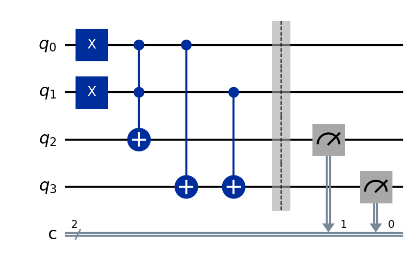

This circuit above shows a Quantum half-adder. We ran this on 2 different platforms, the FakeMarrakesh simulator and the real 156-qubit Heron r2 QPU.

Image("FakeMarakesh_sim_qAdder.png")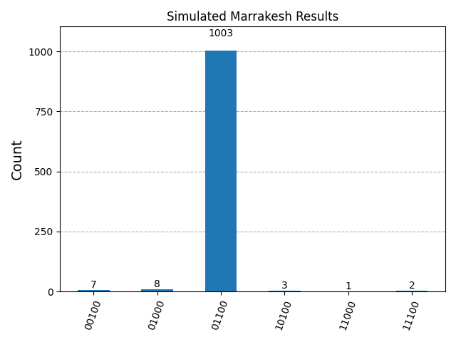

This graph below shows our actual run of the half-adder on the Heron r2.

Image("qAdder_run.png")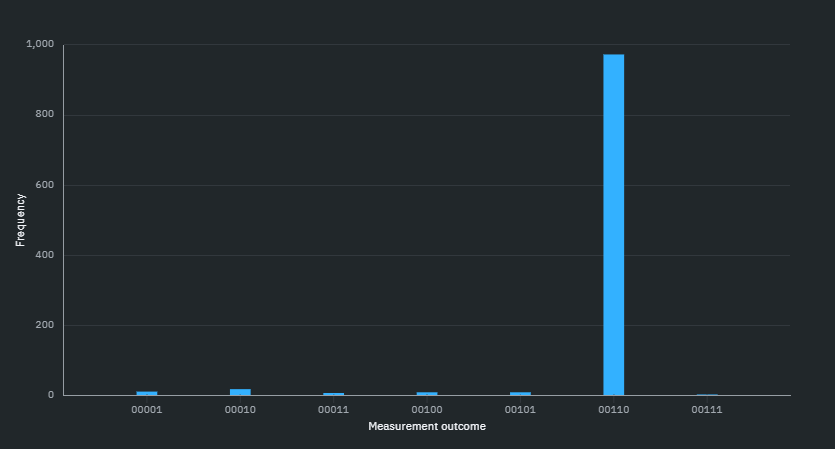

We can see the 00110 lead with 95%, while all other outputs return with less than 17 shots, or 1.6%. A interesting comparison that we can use this data for is to see the development of Qiskit and IBMs hardware. From their initial 5-qubit quantum computer to their now Heron r2 156-qubit QPU, we can see the development and growth. Below is IBMs older version of Grovers Algorithm in a circuit.

Image("grover_circuit_og.png")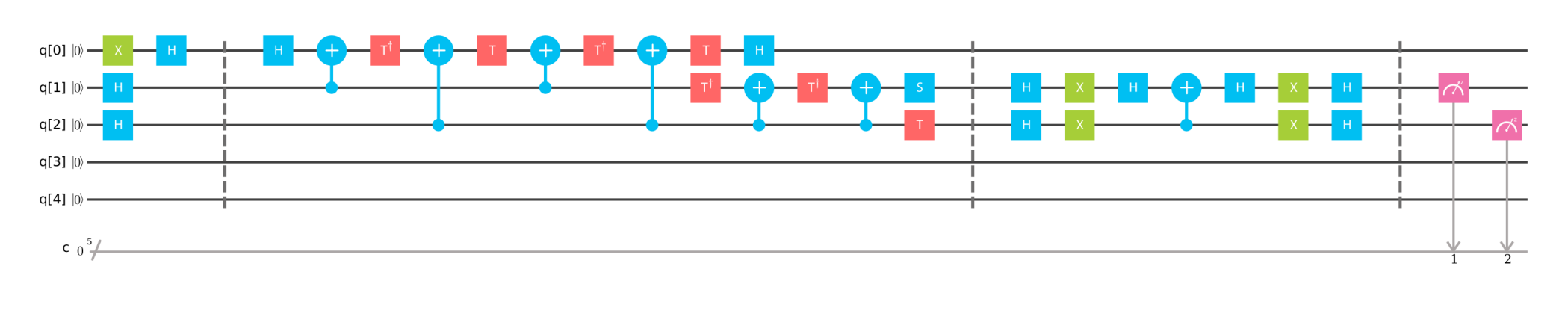

When this circuit is simulated, you get the following.

Image("qAdder_sim.png")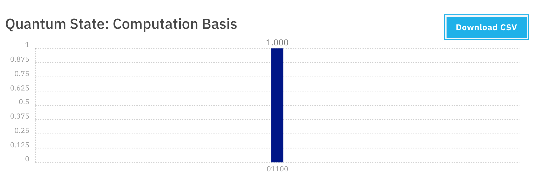

But when sent to IBMs old 5-qubit QPU, the output changes.

Image("qAdder_result.png")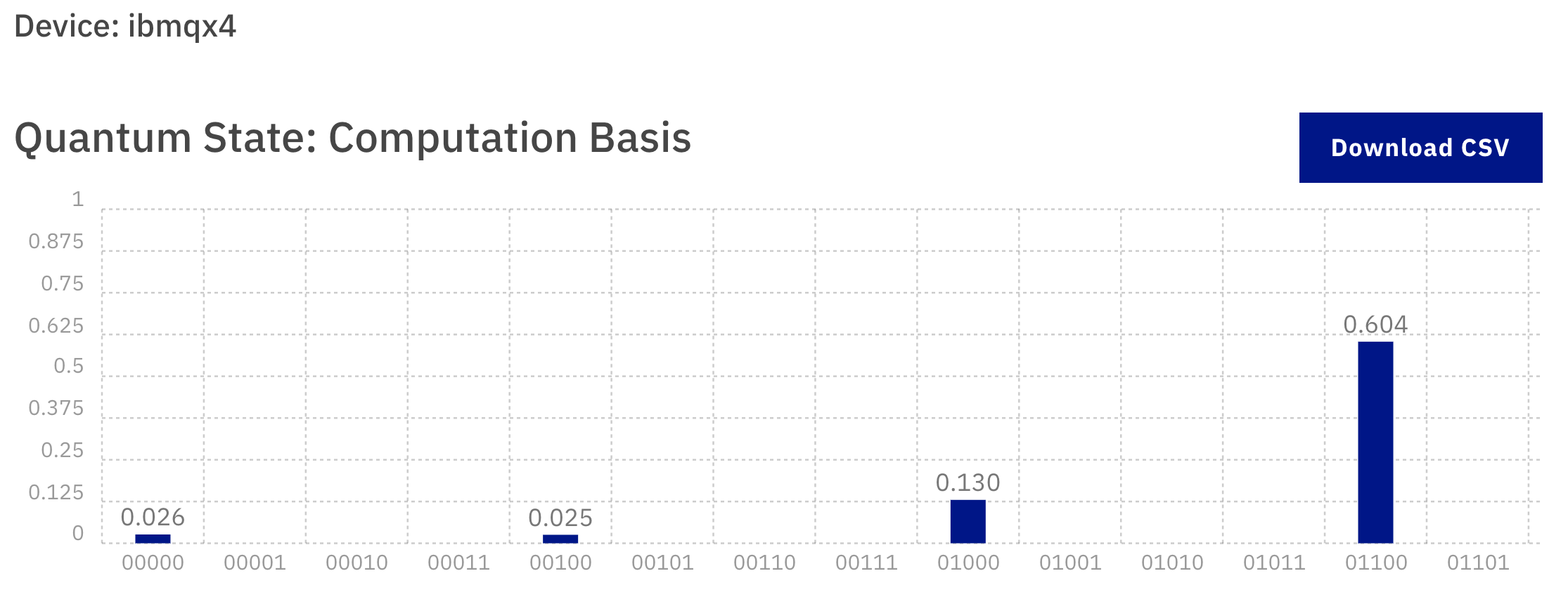

2% difference between simulators while there is a 34.6% difference in the actual runs.

2.2 Grover’s search algorithm¶

The algorithm is first proposed Gover1996 for the search of certain element in an unstructured data base. Given a database with $N$ entries, the algorithm requires only $\mathcal{O}(\sqrt{N})$ operations instead of $\mathcal{O}(N)$ operations of classical algorithms. It is proved optimal later Bennett 1997 on a universal quantum computer.

2.2.1 Grover’s algorithm¶

The core of the algorithm is an oracle (blackbox) to implement such equation, given $x^*$ is the target entry in the database in binary form,

\begin{align} f(x) = \begin{cases} 1, & \mbox{if } x = x^* \\ 0, & \mbox{if } x \neq x^* \end{cases} \end{align}

(19)

where $x$ is arbitrary entry in database.

In addition, the oracle $\hat O$ performs the operation on $n+1$ qubits:

\begin{align} \hat O |x\rangle |q\rangle = |x\rangle | f(x) \oplus q\rangle \end{align}

(20)

where $q$ is an ancillary qubit, and $n$ is the total number digit to represent binary form of total $N$ elements in database. If $x=x^*$ (the oracle operates on target state), and $| q \rangle = |-\rangle = \frac{1}{\sqrt{2}} ( |0\rangle - |1\rangle )$ :

\begin{align} \hat O (| x^*\rangle |-\rangle) &= | x^*\rangle \frac{1}{\sqrt{2}} \left( |f(x^*) \oplus 0\rangle - |f(x^*) \oplus 1\rangle \right) \\ &= | x^*\rangle \frac{1}{\sqrt{2}} \left( |1 \oplus 0\rangle - |1 \oplus 1\rangle \right) \\ &= | x^*\rangle \frac{1}{\sqrt{2}} \left( |1 \rangle - |0\rangle \right) \\ &= -| x^*\rangle |-\rangle \end{align}

(21)

Followed by a mirroring operation $(2|\psi \rangle \langle \psi | - \mathcal{1}_N)\otimes \mathcal{1}$ , where $| \psi \rangle = | + \rangle^{\otimes n}$ is an even superposition of all the $N$ states, and $\mathcal{1}_N$ is the identity matrix of the dimension of $N$ . For an arbitrary state $\sum_i a_i |i\rangle$ ,

\begin{align} (2|\psi \rangle \langle \psi | - \mathcal{1}_N ) \sum_i a_i |i\rangle = \sum_i \left(2 \langle a \rangle - a_i \right) |i\rangle \end{align}

(22)

where $\langle a \rangle = \sum_i a_i / \sum_i 1$ .

The Grover operator $\hat G$ , acting on $n+1$ qubits, is then

\begin{align} \hat G = \{(2|\psi \rangle \langle \psi | - \mathcal{1}_N)\otimes \mathcal{1}\} \hat O \end{align}

(23)

Applying Grover operator is to flip the sign of the coefficient of the target state and then to make the coefficient more than average value of all coefficients. On the other hand, the rest coefficients are decreasing.

The geometric interpretation unfolds as below.

From the initial state being in $| \psi \rangle$ , this Grover operator performs rotation within a subspace spanned by $| \psi \rangle$ and the target state. Now consider the answer space with $M$ targets, and the rest of the Hilbert space represented as

\begin{align} | \alpha \rangle &\equiv \sum _{x^*}^a \frac{N-M}{N}| x^* \rangle \quad \text{orthogonal space}\\ | \beta \rangle &\equiv \sum _{x}^r \frac{1}{M}|x \rangle \quad \text{answer space} \end{align}

(24)

and then the initial state is

\begin{align} | \psi \rangle = \sqrt{\frac{N-M}{N} }| \alpha \rangle + \sqrt{\frac{M}{N}} | \beta \rangle \end{align}

(25)

Then let $\cos \frac{\theta}{2} = \sqrt{ \frac{N-M}{N} }$ , so that $| \psi \rangle = \cos(\theta/2) | \alpha \rangle + \sin(\theta/2) | \beta \rangle$ . The oracle performs a reflection with respect to $| \alpha \rangle$ , since $\hat O (a | \alpha \rangle + b | \beta \rangle) = a | \alpha \rangle - b | \beta \rangle$ , followed by another reflection with respect to $| \psi \rangle$ . Shown in the following figure, applying the Grover operator once is to rotate the initial state to $| \beta \rangle$ with an angle of $\theta$ .

\begin{align} \hat G | \psi \rangle = \cos \frac{3 \theta}{2} | \alpha \rangle + \sin \frac{3 \theta }{2} | \beta \rangle \end{align}

(26)

After repetition for $k$ times, the final state is then

\begin{align} \hat G^k | \psi \rangle = \cos \left(\frac{2k+1 }{2}\theta \right) | \alpha \rangle + \sin \left( \frac{2k+1 }{2}\theta \right) | \beta \rangle \end{align}

(27)

Image("grover_refl.jpg", width=350)
## From Nilsen and Chuang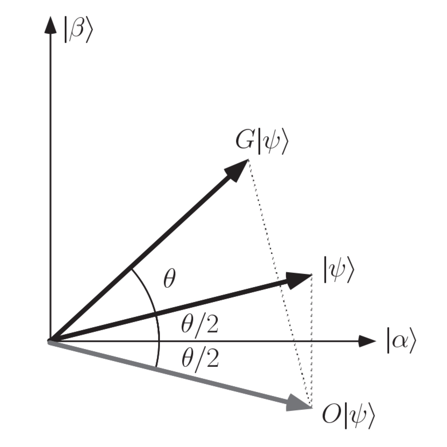

This is to realize amplitude amplification of target state. In the case of $M=1$ , and $N \gg 1$ , $\sin \frac{\theta}{2} = \sqrt{1/N} \approx \theta/2$ , so the rotating angle $\theta = \frac{2}{\sqrt{N}}$ . To reach the target state, the number of applying Grover operator can be calculated as

\begin{align} \frac{2k+1}{2} \theta &= \frac{\pi}{2} \\ 2k + 1 &= \frac{\pi}{\theta} \\ k & = \left(\frac{\pi}{\theta}-1 \right) /2 \\ &\approx \frac{\pi}{4} \sqrt{N} \end{align}

(28)

which means after applying $\hat G$ for the number of $\lceil \frac{\pi}{4} \sqrt{N} \rceil$ times, the amplitude of the target state is close to 1.

2.2.2 Classical simulation of Grover’s algorithm¶

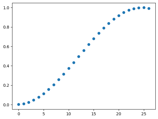
Here, we explicitly calculate the coefficients of the evolving state, to have a simulation of Grover’s algorithm.

## Classical simulation of Grover's algorithm

import numpy as np
import math
import matplotlib.pyplot as plt
%matplotlib inline

n = 10  # num of qubits
N = 2**n  # num of elements
tar = 3 # target element <= N
# max_iter = 100 # total number of iterations
max_iter = math.ceil(np.pi/4*2**(n/2))

psi_0 = np.ones(N) * np.sqrt(1/N) # initial state

F = np.zeros(max_iter+1)
Res = np.zeros(max_iter+1)
F[0] = psi_0[tar-1]**2
Res[0] = psi_0[0]**2

psi = psi_0
for num_iter in range(max_iter):
    psi[tar-1] = -psi[tar-1]  #  flip he target coefficient after Oracle, others remains same
    aver_psi = np.mean(psi)
    psi = 2*aver_psi - psi  # The whole vector goes through the mirroring
    F[num_iter+1] = psi[tar-1]**2
    Res[num_iter+1] = psi[0]**2
#     plt.plot(num_iter,psi[tar-1],'ro')

plt.plot(np.arange(max_iter+1),F,'o')
# plt.plot(np.arange(0,max_iter),Res,'o')
print(F)

[9.76562500e-04 8.76618922e-03 2.42238486e-02 4.71082506e-02
 7.70621756e-02 1.13618051e-01 1.56205248e-01 2.04158992e-01
 2.56730738e-01 3.13099854e-01 3.72386433e-01 4.33665027e-01
 4.95979092e-01 5.58355923e-01 6.19821833e-01 6.79417356e-01
 7.36212219e-01 7.89319871e-01 8.37911315e-01 8.81228051e-01
 9.18593915e-01 9.49425637e-01 9.73241941e-01 9.89671060e-01
 9.98456541e-01 9.99461245e-01 9.92669487e-01]

2.2.3 Implementation of Grover’s algorithm on IBM Q hardware¶

By using IBM’s hardware, its easier to realize Grover’s algorithm. They have a page on their IBM Quantum Platform where you can learn in more depth on the algorithm and how to implement it into your circuits. We can see the full developed Grover’s algorithm circuit shown below

Image("grover_operator.png")

$q_o$ and $q_1$ are the data qubits and $q_2$ is the ancillary qubit. Qiskit has its own simplified version which visually eases the circuit with all the gates. IBM also has an operator of Grovers Algorithm, (grover_op) shown below.

Image("grovers_simp.png")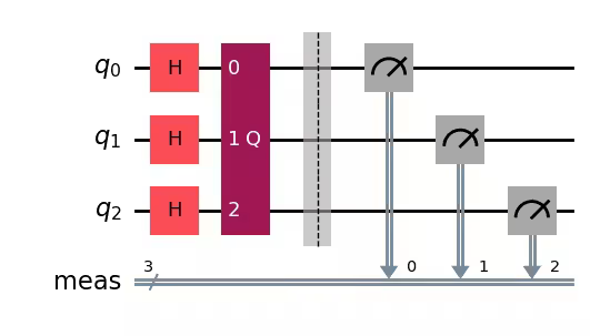

In our case, we will use a more broken down version of Grover’s Algorithm. Going barrier by barrier, we begin by placing our qubits into superposition. We then add in the quantum oracle, followed with a diffusion operator. With those, we essentially have our Grover’s Algorithm . All that’s left is to measure our 2 qubits and see what we get.

Image("Grover_Circuit_new.png")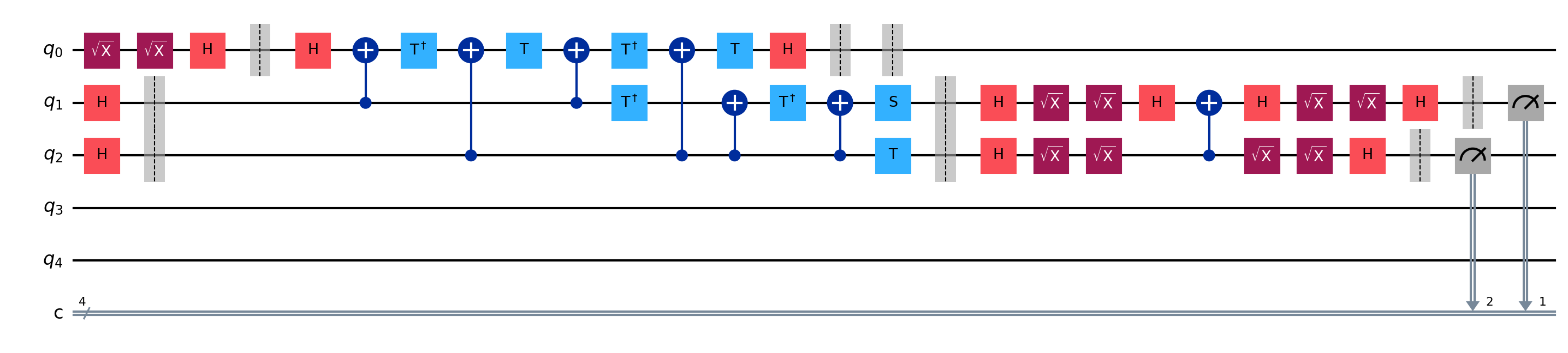

We can run this circuit on a simulator, specifically the FakeMarrakesh 156-qubit quantum computer simulator.

Image("FakeMarrakesh_sim_results.png", width=500)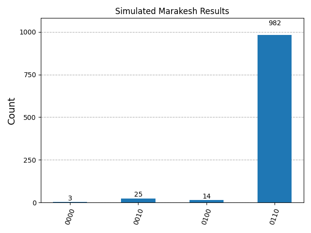

When then ran it on the actual ibm_marrakesh quantum computer, where we can see we get the following:

Image("grover_marrakesh.png")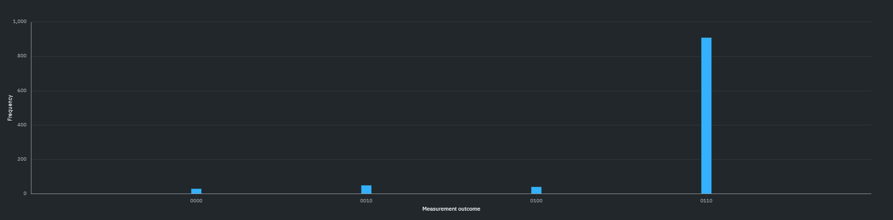

The result in the actual run is 909 out of 1024 shots, or 88.7%, while on the simulated is 982 out of 1024 shots, or 95.8%. We can also compare this data to previous work performed with the same simulator and 5-qubit computer.

Image("grover_circuit_og.png")

Image("grover_sim.png")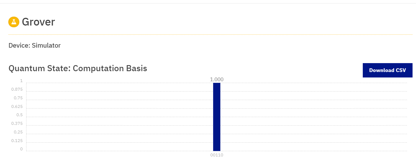

Image("grover_result.png")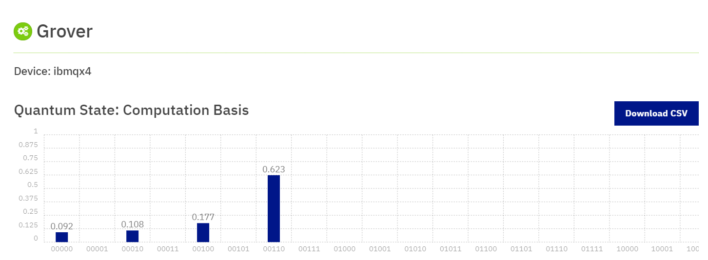

2.2.4 Try It Out¶

The previous examples are a little more complicated, so lets create a 2-qubit system step by step. We'll start by preparing all our libraries.

from qiskit import QuantumCircuit

Next we start building out circuits ‘frame’.

gc = QuantumCircuit(2) # gc = grover circuit with 2 qubits
gc.clear()

Now we want to apply our gates and operations, so we’ll start by applying Hadamard Gates and then a barrier so that our circuit can be processed in the order we want.

gc.h(0) #hadamard to qubit 0 
gc.h(1) #hadamard to qubit 1
gc.barrier() # add a barrier to separate our gate
gc.draw('mpl') # draw the circuit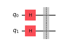

<Figure size 287.294x200.667 with 1 Axes>

We’ll then apply our oracle which will be a Controlled Z-Gate to both qubits.

gc.cz(0,1) # controlled z gate to both qubits
gc.barrier() # barrier to separate them
gc.draw('mpl')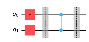

<Figure size 454.517x200.667 with 1 Axes>

Now we add our diffuser.

gc.h([0,1]) # the [] allows us to apply certain gates and operations simultaneously 
gc.z([0,1])
gc.cz(0,1)
gc.h([0,1])
gc.draw('mpl')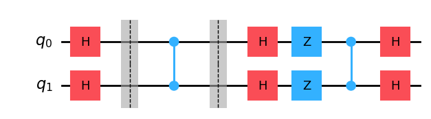

<Figure size 788.961x200.667 with 1 Axes>

And that’s our finished circuit! If we were to run this on a simulator, we’d get essentially the same results as the previous circuit!

3 Summary and Outlook¶

Here I went back for the basic concepts of quantum computing and quantum circuits. We briefly introduce the new system of IBM Quantum Platform and some of its resources. Later, I gave two example of implementing algorithm on IBM hardware. Their 2 new quantum computers allow us to see the evolution of quantum computing.