Introduction to Quantum Computing Through IBM Qiskit - Quantum Computing & Quantum Information

In this section, I will demonstrate how to install the python package, qiskit

1. Prepare By Installing IBM Qiskit¶

There is an instructional on their website: Qiskit. It requires Python version >= 3.5, and “pip install qiskit” for most linux/unix users.

For windows user, I recommend Anaconda to manage python versions and packages. Once installed, you can open “Anaconda Prompt” to launch a terminal-like window to install qiskit.

2. Working with Qiskit¶

You may noticed from the account information page, that using qiskit can access to 16-qubit quantum chips and also to simulate and visualize your circuit. Their website has a straight-forward Qiskit tutorial. From the Qiskit program, we don’t need to take care of the connection problem (for now). The connection of quantum hardware varies and it will be taken care of by the qiskit.

2.1 Examples of Quantum Algorithms¶

2.1.1 Quantum half-adder¶

The quantum half-adder is a working algorithm and fun to start. The circuit is

from IPython.display import Image

Image('quantum_half_adder.png')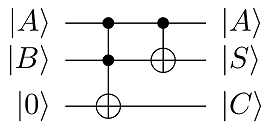

Lets try creating a Quantum Half Adder using the Toffoli Gate (CCX). We’ll start by initializing out qubits.

from qiskit import QuantumCircuit 

qc = QuantumCircuit(4,2) # 4 qubits and 2 classical bits 

#apply NOT gates to the qubits
qc.x(0)
qc.x(1)

#apply our Toffoli Gate (CCX)
qc.ccx(0,1,2)

#draw the circuit
qc.draw('mpl')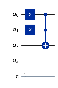

We then measure $q_0$ and $q_1$ each individually with their own CNOT gate, where they flip $q_3$ depending on their values. We end it by measuring both $q_2$ and $q_3$ , where we can then get our binary value.

from qiskit import QuantumCircuit 

qc = QuantumCircuit(4,2)

#apply NOT gates to the qubits
qc.x(0)
qc.x(1)

#apply our Toffoli Gate (CCX)
qc.ccx(0,1,2)

#apply CNOT gate to q0 and q1 
qc.cx(0,3)
qc.cx(1,3)

#apply barrier to whole circuit 
qc.barrier()

#measure qubits 2 and 3 
qc.measure(2,1)
qc.measure(3,0)

#draw the circuit
qc.draw('mpl')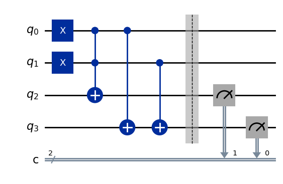

Now lets see what we get when we simulate it and then run it.

Image("Toffoli_qAdder_sim_results.png")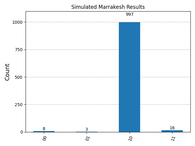

Our outputs here only have 2 digits since we are only measuring 2 qubits instead of all 4. This is relevant since in our actual run with Marrakesh, even though we don’t explicitly measure all the qubits, they are still included.

Image("Toffoli_run_results.png")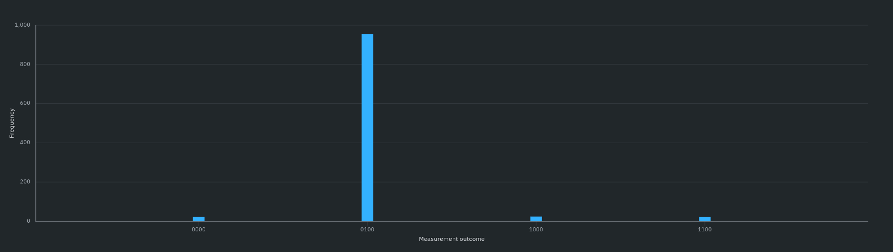

For this data above, we can see that our measurement of 0100 is our highest shot count with 955 shots out of the 1024. Here, our data is arranged as $q_2$ being the first value with $q_4$ being the 2nd digit. So that means that the highest probability would be when $q_2$ is 1 and $q_3$ is 0. Same situation as the simulation, except our values are inverted, so you’d read the output value from top to bottom instead of left to right, so it’d be 01, the same as out run in IBM.

2.1.2 Grover’s search algorithm¶

The Grover’s search algorithm is difficult to build on the web interface. The circuit is then:

Image('grover_circuit.png')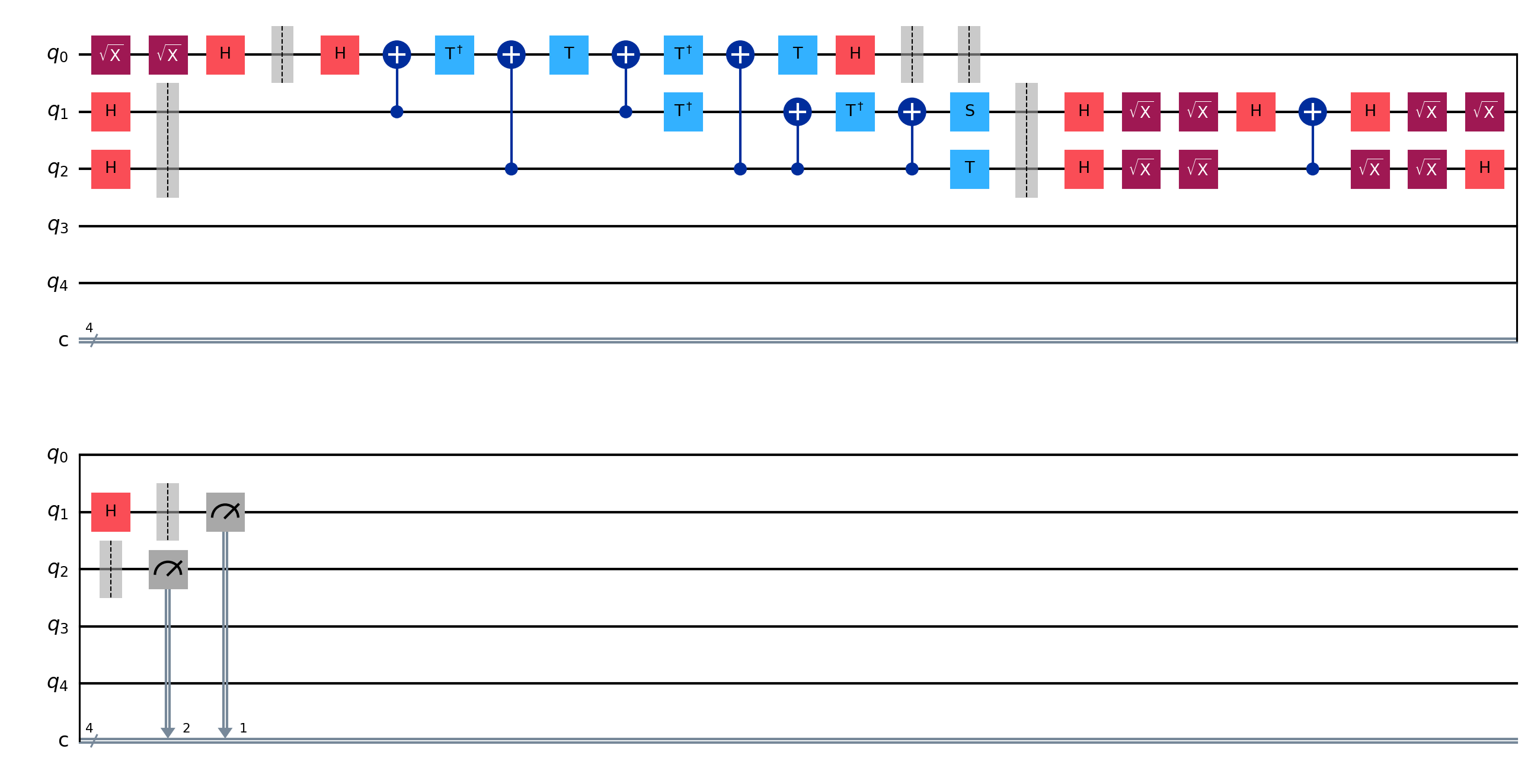

Remember, the second subroutine is the oracle, which is a Toffoli gate to search number 3. Chapter 8 Summary goes deeper into Grovers Search Algorithm.

3. Programming¶

From the tutorial, it is straight forward to build a foundation to simulate/execute a quantum circuit. We can later substitute the core algorithm part for further implementations.

##In case you do not have the libraries, and you are running this notebook, you need to remove the "#" from the lines below:
#!pip install qiskit
#!pip install qiskit-aer
#!pip install pylatexenc

"""
Quantum circuit for quantum half-adder / Grover's algorithm
Updated to be compatible with Qiskit 1.x (2025-06-26)
"""
import math
import matplotlib.pyplot as plt
import matplotlib
matplotlib.use('TkAgg') 
import numpy as np
from qiskit import QuantumCircuit, ClassicalRegister, QuantumRegister
from qiskit_aer import AerSimulator
from qiskit import transpile
from qiskit.visualization import plot_histogram

# Parameters
num_qubit = 5
qr = QuantumRegister(num_qubit, 'qr') # Create a quantum register called "qr" with " num_qubit" qubits
cr = ClassicalRegister(num_qubit, 'c') # Create a Quantum Circuit
qc = QuantumCircuit(qr, cr) # Create a Quantum Circuit called "qc". involving the Quantum Register "qr"

# Quantum half-adder
##### Initial state
qc.x(qr[0]) # qr[0] represent the first input bit set to 1
qc.x(qr[1]) # same as qr[0], after the quantum algorithm, it is then the sum
# qr[2] is the carry bit.

##### Start of the quantum circuit #####
qc.ccx(qr[0], qr[1], qr[2])
qc.cx(qr[0], qr[1])

<qiskit.circuit.instructionset.InstructionSet at 0x1dcccc1b160>

# Grover's search 

##### Initial state
qc.x(qr[0])
qc.h(qr[0])
qc.h(qr[1])  # qr[1] and qr[2] are the output
qc.h(qr[2])

## Grover's operator
### The Oracle to find 3 in {0:3}
qc.ccx(qr[1], qr[2], qr[0])

### Flip
qc.h(qr[1])
qc.h(qr[2])

qc.x(qr[1])
qc.x(qr[2])

qc.h(qr[1])
qc.cx(qr[2], qr[1])
qc.h(qr[1])

qc.x(qr[1])
qc.x(qr[2])

qc.h(qr[1])
qc.h(qr[2])

qc.h(qr[0])
qc.x(qr[0])
### END of quantum algorithm


qc.draw('mpl')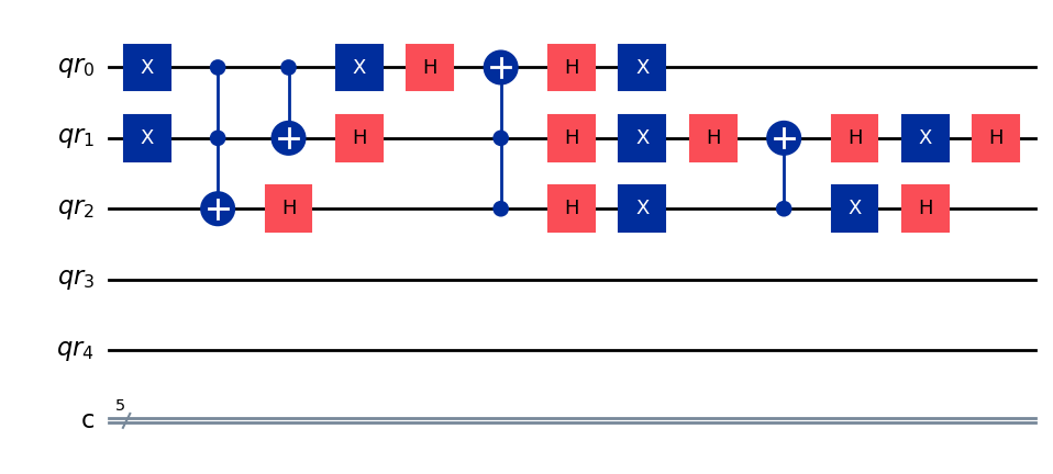

<Figure size 1219.24x535.111 with 1 Axes>



qc.barrier() 
qc.measure(qr, cr) # map the quantum measurement to the classical bits

# Simulation
simulator = AerSimulator()
compiled = transpile(qc, simulator)
job = simulator.run(compiled, shots=8000)
result = job.result()  # Grab the results from the job.
counts = result.get_counts()
print("Simulation result:", counts)

plot_histogram(counts).show() #perhaps you need to run this twice to see the histogram
#plt.savefig("histogram.png")

Simulation result: {'00101': 1981, '00011': 1991, '00001': 1971, '00111': 2057}

#in my run I got

Image('sample.png')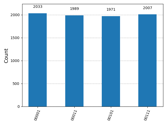


# Circuit visualization
fig = qc.draw('mpl')
fig.show()

#in my run i got

Image('sample2.png')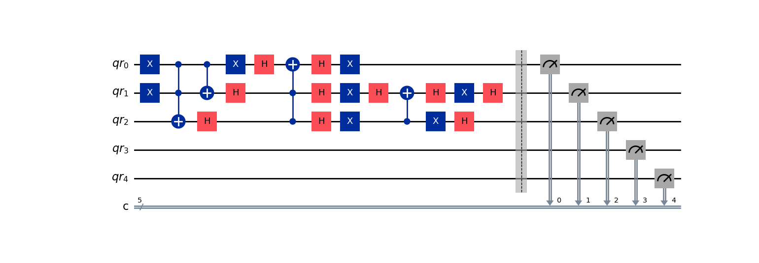

Try to play with the circuit to realize 0+1 and search number 2 in the database {0:3}

Does the naming of the qubits effect the implementation results? How different are the result using qiskit and using web interface?

Optimizing the circuit? For example, HXH=Z, which means we can reduce the number of quantum gates.

We can also see what a run on 156-qubit QPU would look like below

Image("sample3.png")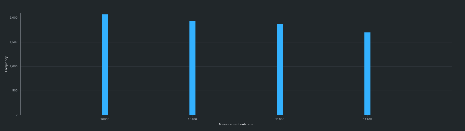

2073 shots for 10000, 1934 for 10100, 1876 for 11000, and 1703 for 11100.Compared to the previous graph, we can see once again how the output values are inverted, with out highest shot count bring with 10000 and the highest shot count being 2033 for 00001, same value, just inverted.

4. Open Questions¶

Up to now, the IBM Q team is continuing developing this package to tackle more complex problems. However, with only the basic of qiskit, we are able to design, to simulate and to implement quantum algorithms. The poor performance of the implementation of quantum algorithm still needs deep understandings of errors and optimizations of circuits.

5. Resources¶

The composer: IBM Quantum Platform Composer
The python package: Qiskit
Basic architecture of quantum gates: IBM Q tutorial of basic gates
The Qiskit tutorial: Qiskit tutorial
Trouble shooting for Qiskit: Qiskit Document