Introduction to Quantum Computing and Topics about Quantum-Assisted Machine Learning Through D-Wave - Quantum Computing & Quantum Information

1 Introduction and Preperation¶

Quantum computing is one approach to obtain answer that classical conventional computer cannot easily handle or intractable at all. Using the power of superposition and entanglement (will explain later) of quantum system, quantum algorithms have the potential to provide speed-up (exponential or quadratic) over classical algorithms. For now, the existing quantum devices are not identified as universal quantum computer, but have their own advantages over conventional computers. The topic about quantum-assisted machine learning is also drawing attentions from different aspects.

1 .1 Qubit¶

In general, any two-level quantum system can be treated as qubit, which can be in either quantum state of $|0\rangle$ and $|1\rangle$ . Similar to classical bits (eg. on/off, high voltage/low voltage as 0/1), there are lots of systems that can realize such quantum systems such as the spin of atoms or electrons (up/down), or the occupation number of fermions in optical lattices (0/1). Quantum computing methods have pointed into different directions like trapped-ion, electron on helium, optical lattices, and photonic.

We mentioned the states $|0\rangle$ and $|1\rangle$ as :

| 0 \rangle = \begin{pmatrix} 1 \\ 0 \end{pmatrix} \qquad |1 \rangle = \begin{pmatrix} 0 \\ 1 \end{pmatrix}

(1)

$| \psi \rangle$ is called a “ket” and $\langle \phi |$ is called a “bra”. They are related through $\langle i | = | i \rangle^\dagger$ . These states form an orthonormal basis of the Hilbert space $\langle i | j \rangle = \delta_{i,j}$ . These are all part of the Dirac Notation, which you can learn more about in Chapter 1.

1.2 Pauli Matrices¶

The Pauli matrices, defined as below, is a set of unitary ( $U U^\dagger = U^\dagger U = \mathcal{I}$ ) and Hermitian ( $U^\dagger = U$ ) $2\times2$ complex matrices.

\sigma_x = \begin{pmatrix} 0 & 1 \\1 & 0 \end{pmatrix} \qquad \sigma_y = \begin{pmatrix} 0 & -i \\i & 0 \end{pmatrix} \qquad\sigma_z = \begin{pmatrix} 1 & 0 \\0 & -1 \end{pmatrix}

(2)

1.3 Superposition of quantum states¶

One quantum state can be written as the superposition of other quantum states with complex coefficients. The interpretation is to represent this state in another orthonormal space.

|\psi\rangle = \sum_i \alpha_i |\phi_i \rangle

(3)

Another important set of states to know is the superposition of $| 0 \rangle$ and $| 1 \rangle$ , shown as

| + \rangle = \frac{1}{\sqrt{2}} \left( |0\rangle + |1\rangle \right) \qquad | - \rangle = \frac{1}{\sqrt{2}} \left( |0\rangle - |1\rangle \right)

(4)

which are eigenstates of Pauli-X matrix.

1.4 Bloch Sphere¶

The bloch sphere is one way to visualize the state of one qubit. A general state of one qubit can be written as,

| \psi \rangle = \cos(\theta/2) | 0 \rangle + \sin(\theta/2) e^{i \phi} | 1 \rangle

(5)

from IPython.display import Image 
Image ("blochsphere.png", width=500)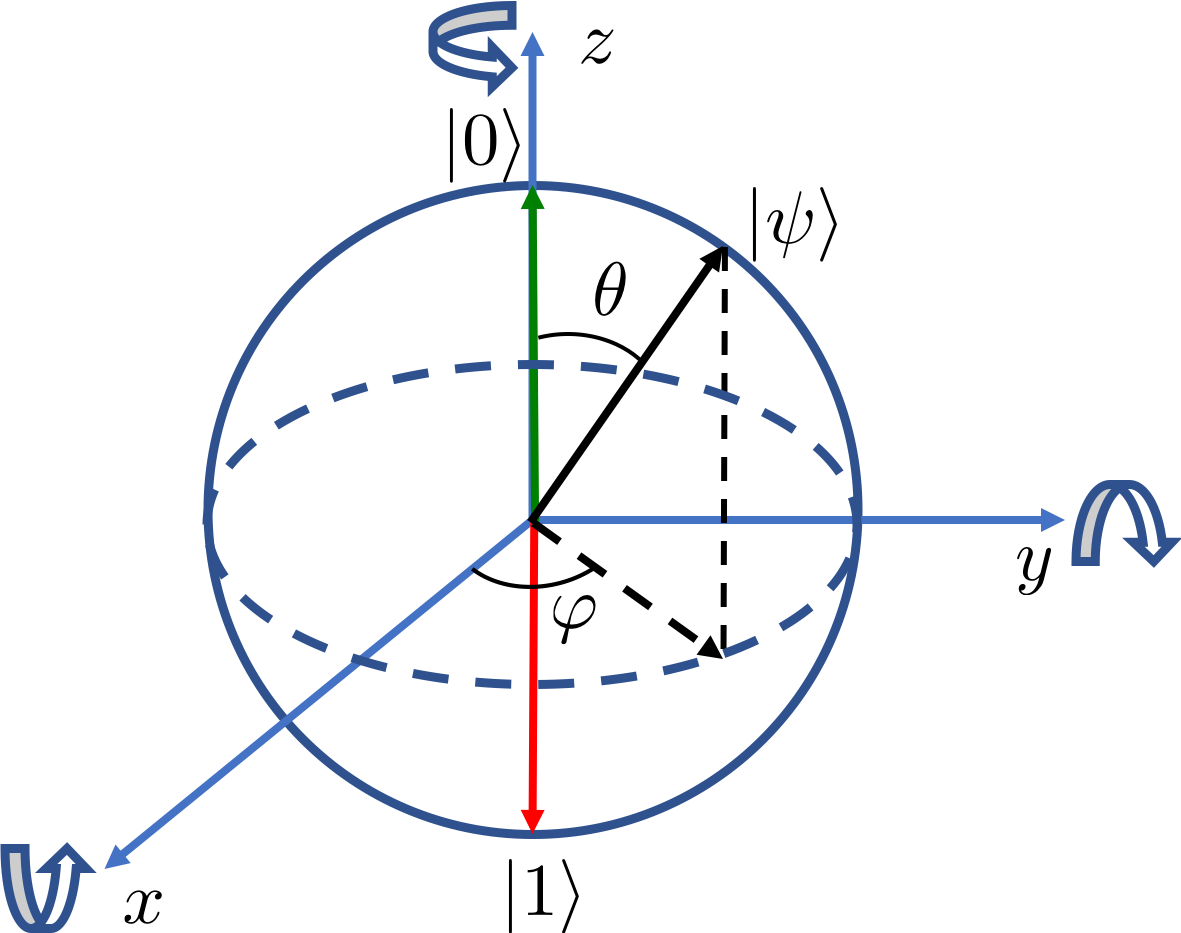

where the $| + \rangle$ and $|- \rangle$ states sit on the X-axis. Chapter 2 looks a little deeper into qubits, states, and the bloch sphere.

1.5 Entanglement¶

Entanglement is a quantum feature of a system of multiple qubits. A entangled state cannot be separated, which means the system cannot be expressed as two independent subsystem.

| \psi \rangle \neq | \psi_A \rangle \otimes | \psi_B \rangle

(6)

One example of entangled states is a Bell state:

| \psi \rangle = \frac{1}{\sqrt{2}} \Big( | 0_A 0_B \rangle + | 1_A 1_B \rangle \Big)

(7)

1.5.1 Density operator and von Neumann entropy¶

The density operator is useful to describe a statistical system in general. It has the definition as

\rho = \sum_i^n p_i | \psi_i \rangle \langle \psi_i |

(8)

where $n \ge 1$ , and $p_i$ is the probability of being in the state of $| \psi_i \rangle$ . When $n=1$ , the system is consider a pure state, or a mixed state otherwise. The trace of a density matrix is always one $tr(\rho)=1$ , and a pure state also satisfies the condition that $\rho = \rho^2$ .

The von Neumann entropy is defined as,

S_{vN}(\rho) = - tr(\rho \ln \rho)

(9)

and it is easy to prove that the entropy of a pure state is zero.

The entropy of a subsystem is also related to measure entanglement to the rest of the system. To obtain the density matrix of a subsystem, we can “trace over” the rest of the system (sometime called environment). Consider a system $\rho$ , consists two subsystem A and B.

\begin{align} \rho_A &= tr_B (\rho) \\ &= \sum_j^{dim(B)} \langle \phi_j | \rho | \phi_j \rangle \end{align}

(10)

HW: Prove a non-entangled state, in the form of $| \psi \rangle = | \psi_A \rangle \otimes | \psi_B \rangle$ , has a density operator of the subsystem A as $\rho_A = | \psi_A \rangle \langle \psi_A |$ , and the entropy is zero.

For an entangled state like a Bell state, $| \psi \rangle = \frac{1}{\sqrt{2}} \Big( | 0_A 0_B \rangle + | 1_A 1_B \rangle \Big)$ , the density operator of system is:

\begin{align} \rho &= | \psi \rangle \langle \psi | \\ &= \frac{1}{2} \left( | 0_A 0_B \rangle \langle 0_A 0_B| +| 0_A 0_B \rangle \langle 1_A 1_B| +| 1_A 1_B \rangle \langle 0_A 0_B| +| 1_A 1_B \rangle \langle 1_A 1_B| \right) \\ \rho_A &= \langle 0_B | \rho | 0_B \rangle + \langle 1_B | \rho | 1_B \rangle \\ &= \frac{1}{2} \left( | 0_A \rangle \langle 0_A | + | 1_A \rangle \langle 1_A | \right) \end{align}

(11)

thus, the von Neumann entropy is $S_{vN}(\rho_A) = - 1/2 \ln (1/2) - 1/2 \ln (1/2) = ln 2$ . Learn about entangled states vs. product states and more in Chapter 3.

1.6 Quantum Gates¶

1.6.1 Single-qubit gates¶

A unitary matrix acts on one qubit is called single-qubit operation, or single-qubit gate. It is considered a rotation of a vector on Bloch sphere, transfer the state vector to a new position. For example, the Hadamard gate, expressed as below, transfer between $| 0 \rangle \leftrightarrow | + \rangle$ , and $| 1 \rangle \leftrightarrow | - \rangle$

H = \frac{1}{\sqrt{2}}\begin{pmatrix} 1 & 1 \\ 1 & -1 \end{pmatrix}

(12)

which can be consider as a rotation with respect to $45^\circ$ axis on X-Z plane.

Applying a gate that is unitary and Hermitian twice in a row will always gives you the identity matrix, and this feature can be used to simplify the circuit to prevent error of implementation.

1.6.2 Two-qubit gates¶

The operation acts on two qubits are always commonly used in quantum circuits. Utilizing two-qubit gates and single-qubit gates, an arbitrary quantum operation on multiple qubits can be approximated to an arbitrary accuracy, and those sets of gates are considered universal. One type of two-qubit gates plays an important role, controlled gate. A controlled gate, using one qubit as the control qubit and determine an operation on the target state. The operation will apply to the target state only if the control qubit is in $|1\rangle$

{}^{c}U|0a\rangle = |0a\rangle \qquad {}^{c}U|1a\rangle = |1\rangle U|a\rangle

(13)

I will introduce one important two-qubit gate, controlled-Not gate (CNOT).

\rm{CNOT} | 0 a \rangle = | 0 a \rangle \qquad \rm{CNOT} | 1 a \rangle = | 1 \bar{a} \rangle

(14)

HW: Try to prepare a Bell state mentioned above on two qubit, using CNOT. What about a quantum operation that swap the state of two qubit?

1.7 Quantum Circuits¶

Quantum circuits represent a set of sequential quantum gates on qubits to perform quantum computation.

Image("ibm_qAdder.png")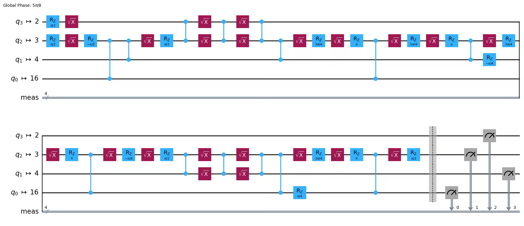

Here is an example of a transpiled quantum half-adder from IBM Quantum Platform Modules. For a broader overview of Quantum Circuits & Gates, take a look at Chapter 4 Summary.

1.8 IBM Quantum Experience¶

The IBM Quantum Platform is an open resource for the public where people can learn quantum computing and building quantum circuits like legos, where you can learn how to build circuits like the one above. IBM also has their Introduction to Qiskit and IBM Quantum, where they teach you how to use their hardware. By using Qiskit, people have access to either their 156 or 127 qubit computers.

2 Hamiltonian Model¶

Aside from a quantum circuit, another model that we can use to conduct quantum computing is the Hamiltonian model. From the Schrodinger equation with time-independent Hamiltonian H:

i \hbar \frac{\partial}{\partial t} | \psi \rangle = \hat{H} | \psi \rangle

(15)

we can consider the system is undergoing a unitary transformation:

| \psi(t) \rangle = \exp \big(-\frac{i}{\hbar} \hat{H} t\big) | \psi(0) \rangle

(16)

For a time-dependent Hamiltonian H(t), the system will undergo a path instead of an arc in Hilbert space.

HW: what is the corresponding equation of motion of density matrix described by the Schrodinger equation?

2.1 Adiabatic Quantum Computing (AQC)¶

Adiabatic quantum computing is based on the adiabatic theorem of quantum mechanics, stating that if the initial state is one of the eigenstate of initial Hamiltonian, the system will remain in that eigenstate if the system undergoes small perturbation. In another expression, if the system is time-dependent and changing slowly that the difference can be treated as perturbations, the system will remain in instantaneous eigenstate of this Hamiltonian.

For example, if the system is in the ground state (lowest energy state) of Hamiltonian H(0), as the Hamiltonian H(t) changes slowly enough, the system is always be in ground state. Here the fidelity is defined as $F(| a \rangle, | b \rangle ) = | \langle a | b \rangle | ^2$ .

## Example of adiabatic state transformation

import numpy as np
from numpy import linalg as LA
from scipy.linalg import expm
import matplotlib.pyplot as plt
%matplotlib inline 

T_total = [1, 2, 10]
dt = 0.001

px = np.matrix([[0,1],[1,0]])
pz = np.matrix([[1,0],[0,-1]])
psi0 = np.matrix([1/np.sqrt(2),1/np.sqrt(2)])
psi0 = psi0.T

for T_tot in T_total:
    q = int(T_tot/dt)
    F = np.zeros(q)
    time_step = np.zeros(q)
    phi = psi0
    for i in range(q):
        H = (1-(i+1)/q)*px + (i+1)/q*pz  
        phi = expm(-1j*H*dt)*phi
        E , VE = LA.eig(H)
        F[i] = (np.absolute(VE[:,0].T*phi))**2
        time_step[i] = i*dt
 
    plt.plot(time_step,F)

In this example, the time-dependent Hamiltonian is written as a linear interpolation of initial Hamiltonian and final Hamiltonian, which is straight-forward and commonly used, but not optimized. The AQC requires several conditions:

The initial state is easy to prepare
The time-dependent Hamiltonian is well-defined
The changing speed of Hamiltonian shall be slow As shown above, if the changing speed is too fast (total ramping time is to short), the final state is far away from correct answer. Depending on the answer encoded in the target quantum state, the AQC can obtain the correct answer for large system problems.

This technique can also be used to prepare a required state for further experiments, known as the adiabatic state preparation.

However, the feature of system staying in the eigenstates can be hard to handle. During the ramping, if the system is excited to another eigenstate, it can be trapped in that state and therefore results in a poor fidelity. An open question is to determine an optimal ramping (other than linear interpolation) with minimal knowledge.

2.2 Quantum annealing and D-Wave system¶

Quantum computing devices have developed at a fast rate in the past few years, showing promising possibilities. For a quantum computer to be practical, it needs to meet certain requirements:

The ability to increase the number of qubits (Scalable Quantum Computer)
Qubits can be well prepared into a arbitrary state (initial condition)
Longer decoherence times than gate implementation time (long life-time of system to perform reasonable number of operations)
Universal Gate Set
The ability to retrieve classical information from qubits

Depending on which of these or other factors that are favored, there are different options that can be chosen from. For instance, a quantum system designed to solve specific problems are usually called a quantum simulator. In this case, we will introduce the quantum annealer from D-Wave for quantum assisted/enhanced machine learning.

2.2.1 The Hamiltonian of D-Wave system¶

The core of the D-Wave system is the AQC. The system has a well defined Hamiltonian as:

H_{dw}(t) = A(t) \sum_i a_i \sigma_x^i + B(t) \left( \sum_i b_i \sigma_z^i + \sum_{i,j} c_{ij} \sigma_z^i \sigma_z^j \right)

(17)

with time-dependent function $A(t), B(t)$ to control the initial Hamiltonian and final Hamiltonian. In their system, $A(0) \gg B(0)$ , and at the “end”, $A(T) \ll B(T)$ .

With the initial quantum state $| + + ... +\rangle$ , which is the ground state of $\sum_i a_i \sigma_x^i$ , the $B(t)$ is tuned up so the system will undergo adiabatic ramping into the ground state of $\sum_i b_i \sigma_z^i + \sum_{i,j} c_{ij} \sigma_z^i \sigma_z^j$ .

In another word, this system is designed to find the minimal value of an energy(cost) function of so-call Ising model:

E_{ising} = \sum_i b_i S^i + \sum_{i,j} c_{ij} S^i S^j

(18)

where $S^i \in \{-1, +1\}$

Users have the control of input data ( $b_i, c_{ij}$ ), and obtain corresponding configurations and energies with desired number of read-outs.

The energy function can be rewritten with a transformation $S = 2t -1$ to have a so-called quadratic unconstrained binary optimization (QUBO) format:

E_{QUBO} = \sum_i b'_i t^i + \sum_{i,j} c'_{ij} t^i t^j

(19)

where $t^i \in \{0, 1\}$ . This energy function covers a commonly used cost function in machine learning:

E = -\sum_i b_i v^i - \sum_i c_i h^i - \sum_{i,j} w_{ij} v^i h^j

(20)

where $v^i, b_i$ are the visible nodes and bias, $h^j, c_j$ are the hidden nodes and bias, and $w_{ij}$ are weights. For a system with n bits, the Hilbert space is 2^n dimensional, and grows exponentially with the system size. In this situation, it is hard to find the ground state efficiently or the conventional classical computer might face memory issue.

2.2.2 Features of D-Wave system¶

As mentioned previously, the D-Wave system is designed to find a configuration which minimize a certain cost function, where the conventional computer finds intractable for large system. The information retrieved from D-Wave calculations are classical (configurations of +1/-1 or 0/1 with the corresponding energy). Another feature of D-Wave is the sampling probability is of Boltzmann distribution, i.e.:

\begin{align} P(E_i) &= \frac{1}{\mathcal{Z}} \exp (- \beta E_i) \\ \mathcal{Z} &= \sum_i \exp (-\beta E_i) \end{align}

(21)

Different from the physical definition of $\beta = 1/k_{B} T$ , the $\beta$ here is corresponding to an effective temperature, or can be considered as a rescaling of energy.

This feature of sampling can help dealing with Restricted Boltzmann machine (RBM) of large system size (large number of visible and hidden nodes).

2.3 Review of RBM¶

The RBM a generative stochastic artificial neural network that can learn a probability distribution over its set of inputs. It is indeed a powerful tool for many problems like supervised learning and clustering. A bipartite graph without connections between same layer (shown below) is demonstrating “restricted” Boltzmann machine.

Image("RBM.png")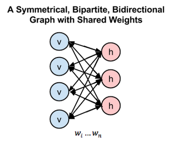

The joint probability distribution of $v,h$ is defined by a Gibbs distribution

P(v,h) = \frac{1}{\mathcal{Z}} \exp(-E(v,h))

(22)

where

E(v,h) = -\sum_i^n b_i v_i - \sum_i^m c_i h_i - \sum_{i,j}^{n,m} w_{ij} v_i h_j

(23)

with $n$ visible nodes and $m$ hidden nodes. The partition function is

\mathcal{Z} = \sum_{\{v,h\}} \exp (-E(v,h))

(24)

the forward and reverse conditional probability distributions for an RBM are both simple sigmoid functions:

P(h_j=1 | v) = sigm(c_j + \sum_i w_{ij} v_i) \\ P(v_i=1 | h) = sigm(b_j + \sum_i w_{ij} h_j)

(25)

With a fixed training data V, the gradient of the log-likelihood with respect to the weights is:

\frac{\partial \log P}{\partial w_{ij}} = \langle v_i h_j \rangle_{data} - \langle v_i h_j \rangle_{model}

(26)

The first term is the clamped expectation with V fixed and can be calculated efficiently. The second term is the expectation value over the joint probability distribution function mentioned before:

\langle v_i h_j \rangle_{model} = \frac{1}{\mathcal{Z}} \sum_{\{v,h\}} v_i h_j \exp (-E(v,h))

(27)

This term is hard to obtain due to the difficulty of sampling all the configurations, Contrastive Divergence is used to compute the expectation value from model and to update the weights and biases.

2.4 Quantum assisted process¶

Combine the need from RBM and the feature from D-Wave sampling, the quantum annealer can be used to compute the expectation value from training model. It is easy to implement this process as the interface of D-Wave library is well connected with Python. The QUBO to feed in to the D-Wave can be defined as:

Q = \frac{1}{\beta}\begin{pmatrix} B & W \\ 0 & C \end{pmatrix}

(28)

where $B$ and $C$ are diagonal matrices with $b_i$ and $c_i$ . $\beta$ is undetermined. The D-Wave will return configurations of vectors in $(n+m)$ dimension, $(v,h)$ . Then the expectation value, $\langle v_i h_j \rangle_{model}$ , can be calculated as,

\langle v_i h_j \rangle_{model} = \frac{1}{N_r}\sum_n^{N_r} v_i^{(n)} h_j^{(n)}

(29)

When tackling a large system, the D-Wave sampling might be performing better calculations.

Example¶

D-Wave has updated their TOS and does not provide API keys to new users, but we are going to instead use dimod, which is a python library used for building Binary Quadratic Models (BQMs). Dimode is part of the D-Wave Ocean SDK. With it, we are going to translate the energy model of a RBM into a QUBO formulation.

Starting with the tools we’ll use:

import sys
import numpy as np
import dimod
import matplotlib.pyplot as plt
import matplotlib.ticker as ticker

For the RBM parameters, we’ll use a 2 visible and 2 hidden RBM.

Symbol	Meaning	Shape
`b`	visible biases	(n_vis,)
`c`	hidden biases	(n_hid,)
`W`	weight matrix	(n_vis, n_hid)
`beta`	inverse temperature — scales the QUBO	scalar

b = np.array([0.5, -0.3])  #our 2 visible 
c = np.array([0.2, 0.4] )   #our 2 hidden 
W = np.array([[0.8, -0.5],[0.3, 0.6]])  #our weights

beta = 1.0

n_vis, n_hid = len(b), len(c)
n_total = n_vis + n_hid

print(f"Visible nodes : {n_vis}")
print(f"Hidden nodes  : {n_hid}")
print(f"Total QUBO variables : {n_total}")

Visible nodes : 2
Hidden nodes  : 2
Total QUBO variables : 4

With that set, we can start to build the QUBO matrix. Using the formula from 2.4, we can map the RBM energy function onto a QUBO as:

Q = \frac{1}{\beta} \begin{bmatrix} \text{diag}(b) & W \\ 0 & \text{diag}(c) \end{bmatrix}

(30)

Variables are ordered as $[v_0, v_1, \ldots, h_0, h_1, \ldots]$

We can visualize the RBM as below

Image("rbm_visualization.png")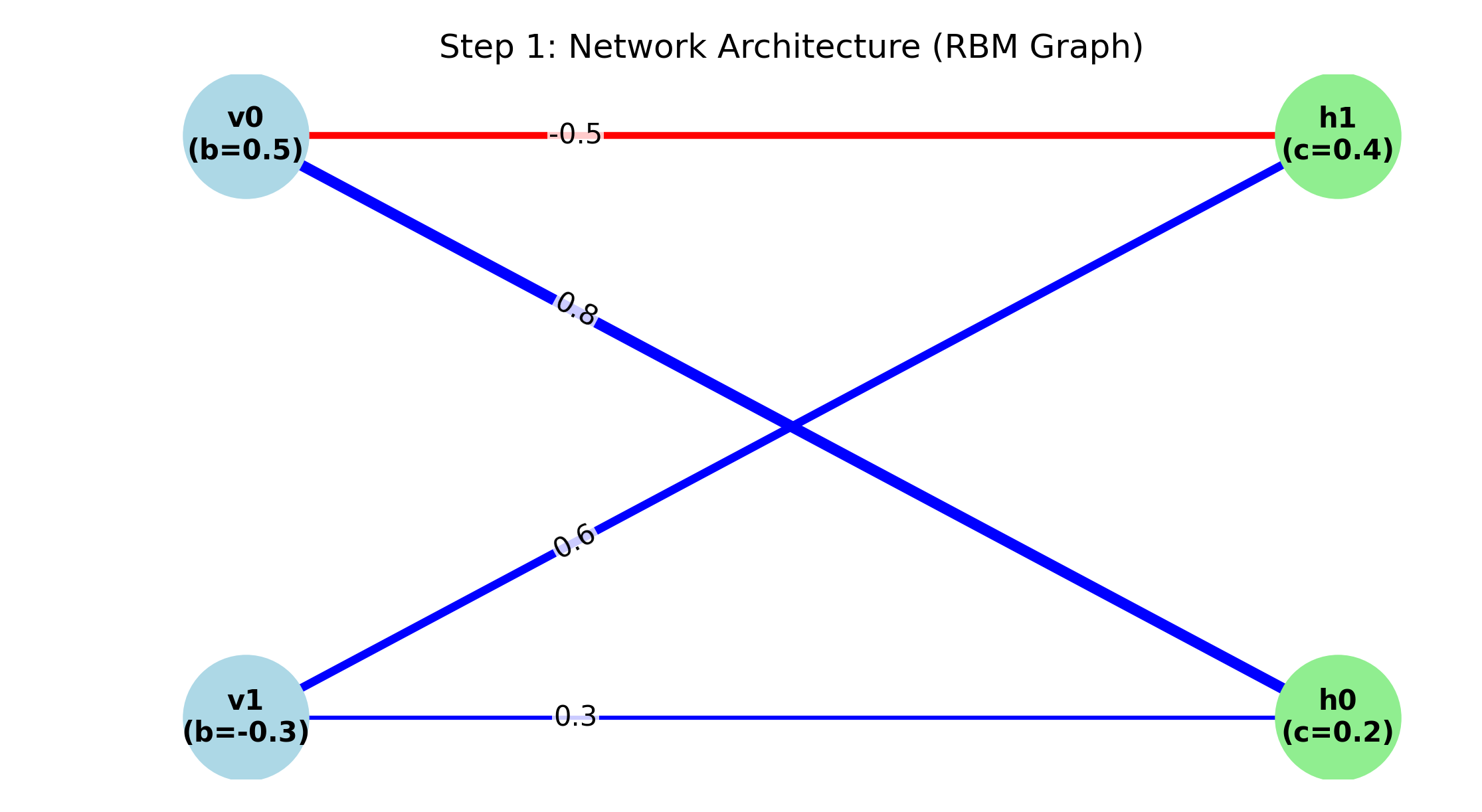

Q_mat = np.zeros((n_total, n_total))

for i in range(n_vis):
    Q_mat[i, i] = b[i] / beta

for j in range (n_hid):
    Q_mat[n_vis + j, n_vis + j] = c[j] / beta

for i in range(n_vis):
    for j in range(n_hid):
        Q_mat[i, n_vis + j] = W[i, j] / beta

Q_dict = {
    (i, j): Q_mat[i, j]
    for i in range(n_total)
    for j in range(i, n_total)
    if Q_mat[i, j] != 0
}

print("QUBO matrix Q (upper triangular, scaled by 1/beta):")
print(np.round(Q_mat, 3))
print(f"\nNon-zero entries in Q_dict: {len(Q_dict)}")

QUBO matrix Q (upper triangular, scaled by 1/beta):
[[ 0.5  0.   0.8 -0.5]
 [ 0.  -0.3  0.3  0.6]
 [ 0.   0.   0.2  0. ]
 [ 0.   0.   0.   0.4]]

Non-zero entries in Q_dict: 8

We can visualize this as a heat map as shown below.

Image("qubo_matrix.png")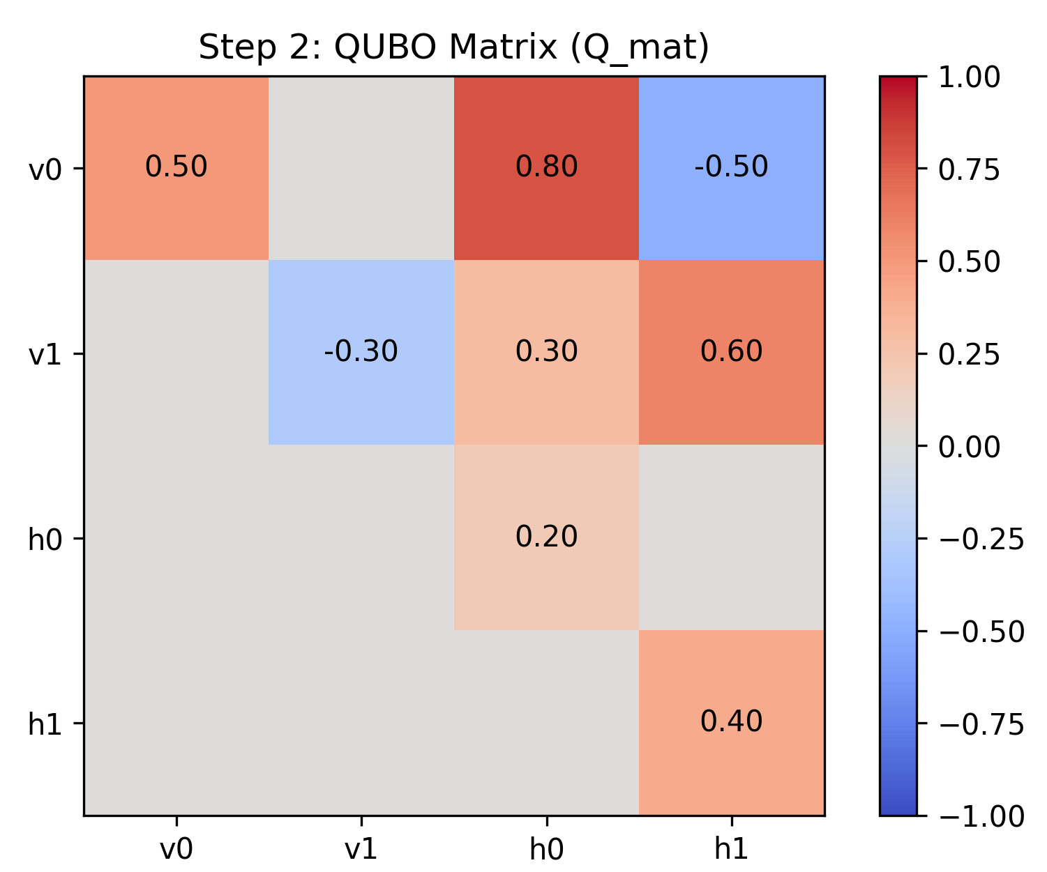

With the QUBO setup, we can start to train the RBM. To do this, we need to know the probability of nodes being active together when the network is allowed to freely settle into its thermal equilibrium.

n_reads = 1000

sampler = dimod.SimulatedAnnealingSampler()
response = sampler.sample_qubo(Q_dict, num_reads=n_reads)

samples = np.array([[s[i] for i in range (n_total)] for s in response.samples()])

print(f"Samples collected : {samples.shape[0]}")
print(f"Variables per sample : {samples.shape[1]}")
print(f"\nFirst 5 samples (columns = [v0, v1, h0, h1]):")
print(samples[:5])

Samples collected : 1000
Variables per sample : 4

First 5 samples (columns = [v0, v1, h0, h1]):
[[0 1 0 0]
 [0 1 0 0]
 [0 1 0 0]
 [0 1 0 0]
 [0 1 0 0]]

With the RBM trained, we can now compute the model expectation.

\langle v_i h_j \rangle_{\text{model}} = \frac{1}{N_r} \sum_{n=1}^{N_r} v_i^{(n)} h_j^{(n)}

(31)

Since both are binary, this equals the fraction of samples where both $v_i$ and $h_j$ were simultaneously active.

v_samples = samples[:, :n_vis]   
h_samples = samples[:, n_vis:]   

vh_expectation = (v_samples[:, :, None] * h_samples[:, None, :]).mean(axis=0)

print("Model expectation <v_i h_j>_model:")
print(np.round(vh_expectation, 4))

for i in range(n_vis):
    for j in range(n_hid):
        print(f"  <v{i}, h{j}> = {vh_expectation[i,j]:.4f}  "
              f"(both active in {vh_expectation[i,j]*100:.1f}% of samples)")

Model expectation <v_i h_j>_model:
[[0.06  0.158]
 [0.127 0.118]]
  <v0, h0> = 0.0600  (both active in 6.0% of samples)
  <v0, h1> = 0.1580  (both active in 15.8% of samples)
  <v1, h0> = 0.1270  (both active in 12.7% of samples)
  <v1, h1> = 0.1180  (both active in 11.8% of samples)

This output is our model expectation, or $\langle v_i h_j \rangle_{\text{model}}$ . Even though we can’t run this on a quantum computer directly, we can still run the math and get a close result with dimod. You can try changing the biases to see how you can get closer to a value you want.

3 Summary and Outlook¶

Here we introduced fundamental concepts of quantum computation of circuit model and Hamiltonian model. Later, we build connection between machine learning and existing quantum devices for a quantum assisted process. There are lots of open questions about quantum computing and potential applications.

References¶

https://blog.csdn.net/Tony_Stark_Wang/article/details/80240060