Assume that you have measured data for motivational purposes and that for each value you have a label. Perhaps you have a list of characteristics of breast cancer samples and the label is 1 (if the cancer is malignant) or 0 (if it is benign) as in Breast Cancer Wisconsin (diagnostic) dataset. Another example is the statistical data of police misconduct in Chicago and the labels are the officer's race as in Citizens Police Data Project. Our main task is to find if we can we make reasonable predictions for the labels of new, unseen data values. The algorithm will return a class based on the algorithm's design and training. The data we use for training it and what we do with the output are choices made by humans; this will have consequences. We recommend to take the 70 minute Fairness Training course to prevent different types of bias on your project.
Preprocessing Data
A big part of the performance of a machine learning algorithm relies on preprocessing the data. If we don't have enough data, or if it is biased, the algorithms will reflect those deficiencies in the output. For example, for the contest and art event Adaptation in 2017, we worked with 3D-scanners until we realized they failed in scanning people of color. The creators of the app suggested that it was an illumination issue, but we claim that deciding that the algorithm is ready, after only testing it on non-colored people at the time, was an error that led the algorithm to be biased. After all, those scanners were used on toys, and the toy-manufacturing companies were not expecting kids to have special illumination while using the toys. An important lesson to obtain from this is that data quality is a priority. Since data is collected by humans, it is important to always look for mistakes by cleaning the data. One of our notebooks "First Machine Learning Notebook" is an excellent guide on data analysis followed by "Higher Dimensions" explains the curse of dimensionality and gives an introduction to higher dimensional geometry.
Which algorithms are we covering?
SVM
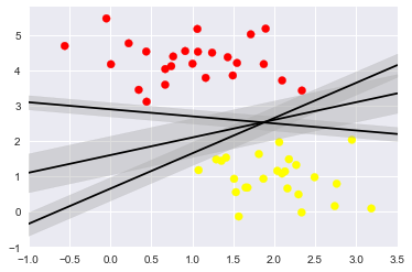
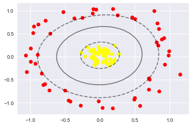
Imagine that you are designing a new material. First you create it in silico, and then you have a team that will materialize those designs. The task is to determine when something could go wrong before investing in completing the material. It is fairly easy to determine what are good properties; however, it is a complex task to imagine what could be bad, especially on a multi scale process. Perhaps the atomic configuration is unstable, the material is below quality, or there is a similar material in properties and quality with a lower price. Since collection of example data of a faulty system can be either expensive or just impossible, there is no way to describe all the possible defects on the material a priori. SVM can be use to attack this kind of problem, as explained in the notebooks. The general idea is explained as follows. Figure 1. Which line shall we choose to separate these points? Assume we are dealing with the classification of labeled data. We have data with information about which class each piece of data belongs to. We want an algorithm to classify new, unseen data. In some cases, it is possible to separate classes using lines, but then the question becomes "Among all possible lines, which one is best to use?" as in Figure 1. Once we have decided how to evaluate quality, we will be able to select a line. A natural requirement is that the algorithm should be robust to new data and minimize the number of misclassifications. In the notebook "Support Vector Machine", you can see how the SVC algorithm looks for the coefficients of such a line. Figure 2. A line cannot separate this data set directly.
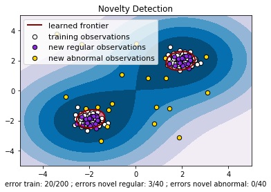
Most real life cases are not linearly separable, but sometimes we can transform the features, hoping that the new features can be separated with hyperplanes. In Figure 2, we added a third coordinate to the data, the distance to the origin. Then in R^3, it is easy to find a plane z=.6 that classifies our data. SVM performs better if we pre-process the data following the rules on the notebook "Cleaning Data". How can we use this algorithm to find anomalies in new products? We can assume that good products have Label 1 and products that are outliers have Label 0. By training the SVC this way, it will learn to classify products either in regular or in outliers. It will recognize when a new product is far from the standard, as in Figure 3. This idea is explained in the notebook "SVC II". Figure 3. Example of novelty detection.
Neural Networks
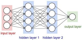
We saw that SVM uses hyperplanes to separate the data, and that sometimes a transformation of the data is needed. In Feedforward neural networks, we use iterations of non-linear functions, followed by matrix transformations that transform data to simplify the classification process. A neural network is a composition of functions of the form where x and b are vectors, W is a matrix, and sigma stands for a non-linear function applied entry wise to the coordinates of the vector W x+b. It is standard notation to represent matrices W as arrows from the domain of x to the domain of w x + b, as in Figure 4. (See the notebook "Neural Network" for details.) Finding the coefficients of those matrices requires Multivariable Calculus and The Chain Rule. In "Keras", you can find an introduction to the software, which we consider the most friendly language in which to use Neural Networks, and gives a deeper explanation of how Neural Networks work and can be trained. An application of Neural Networks to Chemistry can be found in the notebook "Potential Energy Surface ANN", where we describe the work of The Roitberg Group at the University of Florida, a deep, transferable learning potential ANAKIN-ME (Accurate NeurAl networK engINe for Molecular Energies), or ANI for short.
Figure 4. Neural network with two hidden layers. Supposed that you are given input in different steps; for instance, if the input are letters of a name and you want to predict the nationality of the name. To deal with this kind of data, we need to modify our algorithms. Using time just as another variable will result in classification based on when the event/measurement happened. But perhaps we want to find a classification based on classifications previous made on the partial data already registered. The lecture "Recurrent Neural Networks" deals with networks designed for modeling this sequential data. This can be used to make numerical simulations of partial differential equations and ordinary differential equations; we included an example of Character-Level classification of names in "Recurrent Neural Networks II" using Pytorch.
CNN
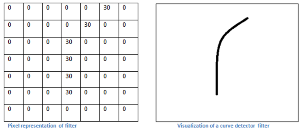
Given a picture of a stocked shelf in a warehouse, a neural network can immediately identify any products that are running out and restock them. The Chinese government are known to have been able to use face recognition to identify fugitives at a music concert. In order to work with images, we would need to solve a problem; images are represented by pixels and a small image would have too many pixels. You would go to your favorite browser and look for images with exactly 500x500 pixels; which would be 250,000x3 numbers. Since we would have to select Red, Green and Blue for every pixel, Feedforward neural networks would require you to find multiples of that many coefficients. Besides that, we would not be working with vectors anymore, as the pixels are related to the pixels in their neighborhood. We would need to change the vectors input to matrices input, and the vectors output to matrix output. You can think of a matrix as a vector with vector entries. Now, the matrices are not only operations, but the elements we work on as well. The good thing about image processing is that we have visuals to help us understand the classification process. We are going to learn smaller matrices called filters, which may be able to learn geometric concepts as a curve or a square (See Figure 5). Figure 5. Pixel representation and visualization of a filter.
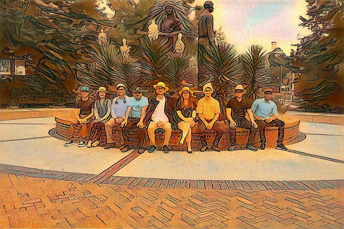
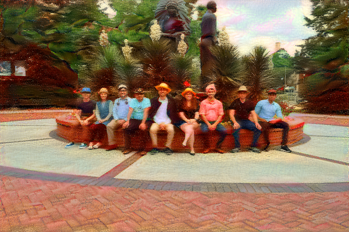
We have a post written by a guest from AI Academy titled "CNN" where we explain in further detail how CNN works. In the lecture "Deep Dreams", we ask the neural network if it recognizes a pattern on an image and then we modify that image to show the pattern. In "Style Transfer", we learn styles of images and mimic its style to other images. For example, in Figure 6, we used a picture of our team and we added the artistic style of the famous Colombian painter Fernando Botero. Figure 6. Style transfer of Botero's paint into our group picture. "Generative Adversarial Networks" describe a generative method. For example, we might have a database of pictures of different clothes, such as the clothes shown in the Fashion-Mnist database, and so we want to generate artificial images as seen in the Ghost Wardrobe project. We can also train GANs with images of people and obtain faces of nonexistent people , or we can also train GANs with images of anime character profiles and obtain new anime character faces. While it is hard to train a GAN, it produces interesting results as shown in this GAN-Paint project or in this password-cracking tool. We recommend reading an arXiv.org article titled "Why does deep and cheap learning work so well?". The authors who wrote this article use physics to try to explain the way neural networks are capable to make classifications.
Bayesian methods
In the notebook "Frequentist vs Bayes", we introduce Bayesian methods and show how they differ from a frequetist perspective. We wish to quantify the accuracy of our predictions frequently; Bayesian methods could provide us a closer estimate of our accuracy. In the "MCMC" lecture, we find a Bayesian approach--one in which we consider the values of the parameters as random variables. Recall Bayes' theorem for training parameters The integral on the bottom is generally not analytic and, due to higher dimensional problems, infeasible to calculate. However, by using the Monte Carlo Markov Chain algorithm, it is possible to make estimations. This algorithm is also useful to study the Ising model, which was created to describe both magnetic and ferromagnetic materials. We also introduce "Simulated Annealing" and "Uncertainty Quantification".
SOM
The Self-Organizing Maps technique is a method that allows us to do dimensional reduction. The main step of the method is to place points randomly and let those points get attracted to the data points in such a way that clusters will pull the points harder. One would then expect the points to end up being placed in the center of the clusters. We expand on this technique in the lecture "SOM". In Figure 7, we can see an image that has been generated using Self-Organizing Maps. Figure 7. SOM in art.
Genetic Algorithms
A genetic algorithm is a search heuristic inspired by Charles Darwin’s Theory of Natural Selection. They reflect the process of natural selection where the fittest individuals are selected for reproduction in order to produce the next generation. Genetic Algorithms are most commonly used in optimization problems, where we have to either maximize or minimize a given objective function value under a given set of constraints. GAs are also used to characterize various economic models like the cobweb model, game theory equilibrium resolution, asset pricing, etc. They also have been used to plan the path which a robot arm takes by moving from one point to another. We can find more applications in multimodal optimization in which we would have to find multiple optimum solutions.
Given a problem we define a fitness function that measures how good is a proposed solution. The higher the fitness the closer to an ideal solution of the problem.The process of natural selection starts with the selection of fittest individuals from a random population, we then select a percentage of the remaining population. This new smaller population go on to produce offspring, mixing genes that seem useful to solve our problem. To explore new genes, we mutate a small percentage of the offspring and add foreigners to obtain the new population. By doing this process several times, the maximum value obtained by the fitness function of the population cannot decrease as every new generation has the fittest individuals of the previous generation, while the mutations and foreigners help us avoid fixed points that are not minimums. For more details see the notebook "Genetic Algorithms" and the notebook "GARFfield" where an application to reactive force fields is explained.
Decision Trees
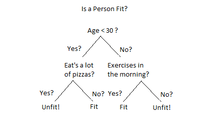
In Figure 8 Figure 8. Example of a decision tree. we asked several questions to determine an algorithm that could tell us whether or not a person is fit, based on their replies. The questions are not necessarily optimal ones, but this illustrates the general methods. We split data points into subsets based on the values on certain features. The order in which we choose the features give us different algorithms. You can find an implementation of this in the notebook "Decision Trees", where we aim to find the best features to consider in the decision.
KNN
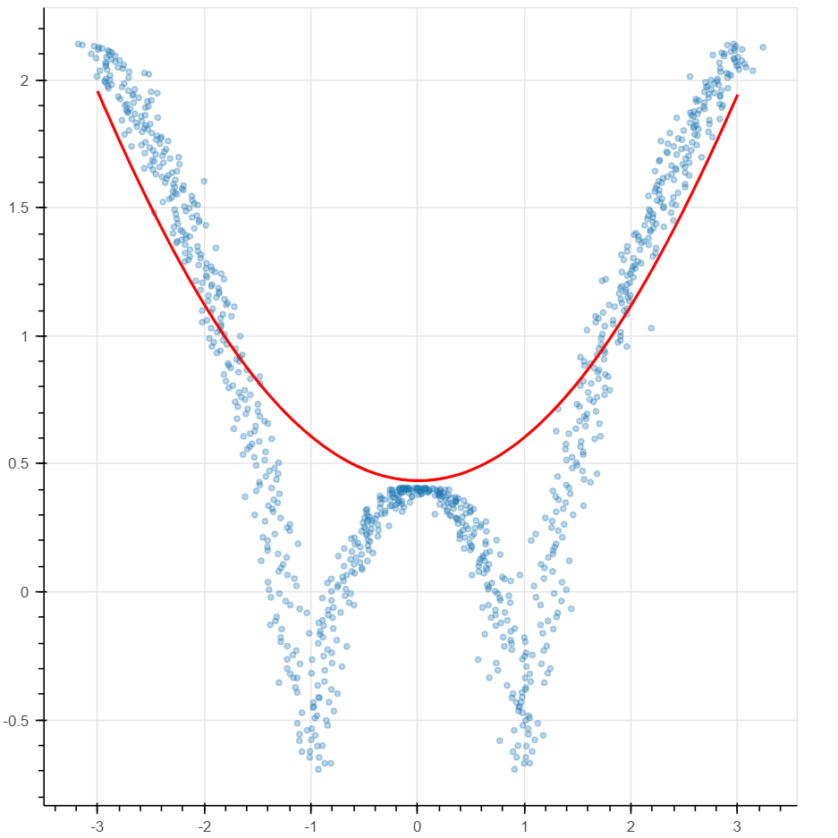
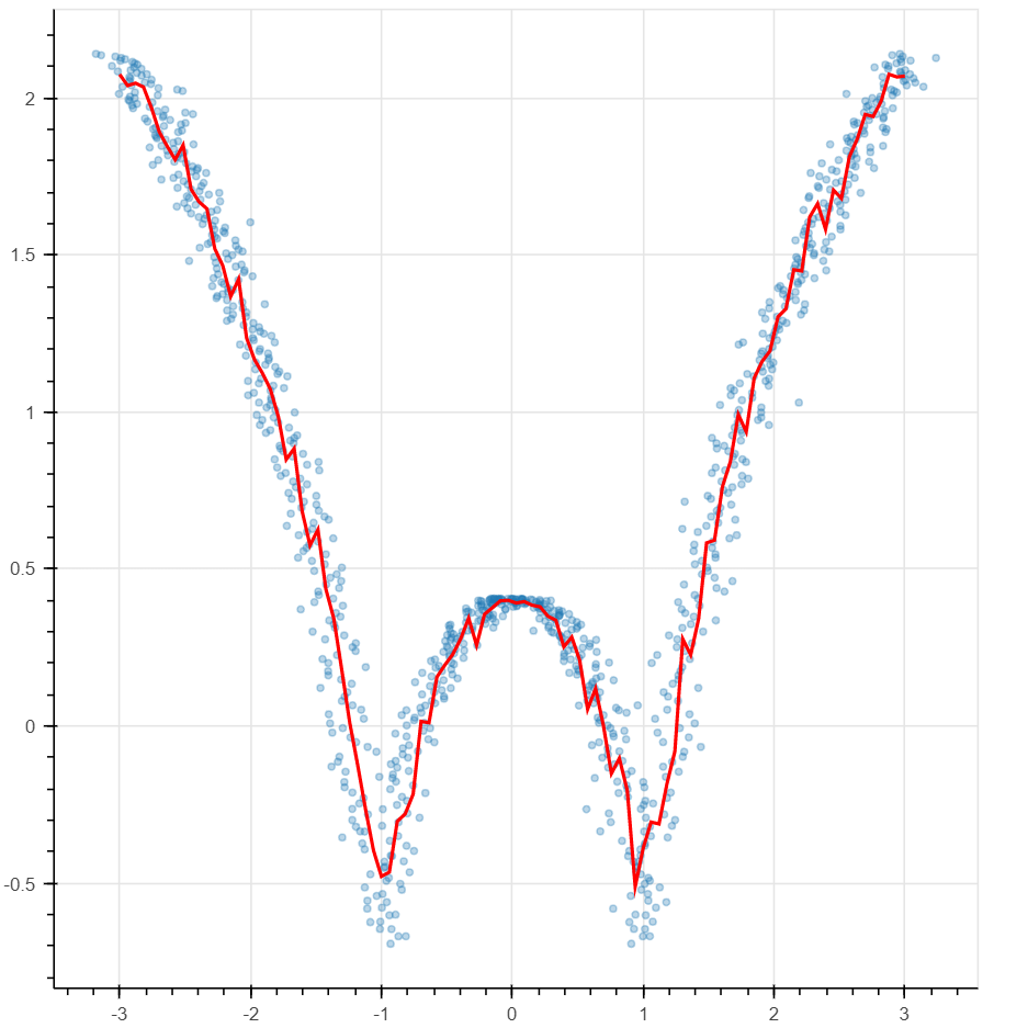
Using the "K-Nearest-Neighbors" algorithm, we can make a prediction or classify an element by only analyzing a neighborhood of the element an assigning to it a function of this neighborhood's values. For example given a new point x and the closest k points to x, you can assign the average of x's neighbor's values to x. K stands for how many nearby points you could consider to make your choice. The results depend on a good selection of the parameter K. If the boundary is a concern, Kernel Regression assigns different weights to the nearby points so that points that are closest matter most. Locally weighted polynomial regression is a local version of polynomial regression where we find the best line or curve that approximates the local NBH. The possibility to write a model that deals with the local picture is important in applications. In Figure 9, we demonstrate examples of locally weighted polynomial regression. Figure 9. Locally weighted polynomial regression.
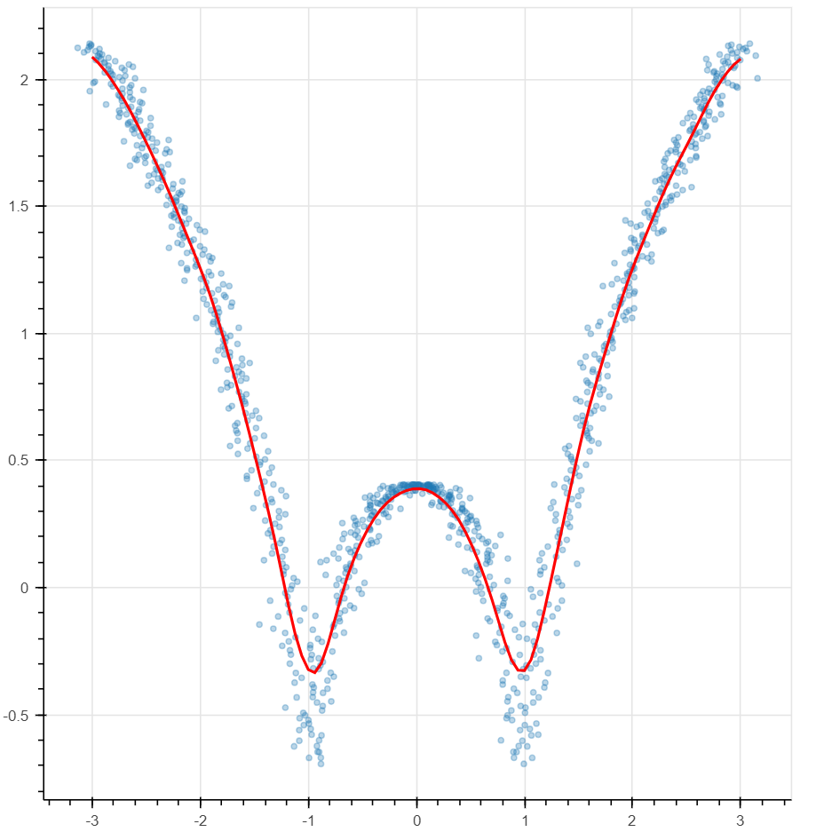
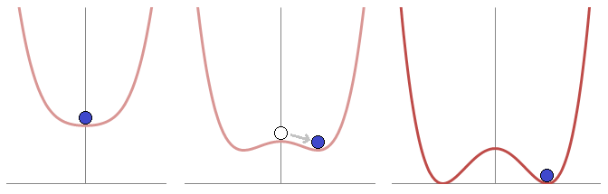
This should remind us of the typical diagrams shown in phase transition, such as the Mexican hat potential, demonstrated in Figure 10. Figure 10. Mexican Hat.
Non Negative Tensor Factorization
We consider data in the form of a matrix. For example, given a vocabulary with m words and n documents, V_{ik} is the number of times the i -word in the dictionary appears in the k document. A database of fixed-sized, grayscale images can also be described by a matrix V. We relabel the pixels in an image form 1 to m, and assume the database has n images. The value of the V_{ik} is the intensity of the i-pixel in the k image.
Non-negative matrix factorization is a process that is used to find two matrices with non-negative entries W,H, so that V approximates W x H. It turns out that the columns of H can be understood as a basis whose linear combination approximates the columns of V. W give us the coefficients so that a juxtaposition of the H columns can recover the initial data. Columns of H have been recognized as eigen images.
Imagine that for every patient you have a matrix of diagnoses and medications. We can label columns with different medications, and label rows with different diagnoses. The entries would be mostly zeroes, except for when the patient would be diagnosed with the i-sickness and received the k-medication. If we stack these matrices on top of each other, we would then have a 3-dimensional matrix, or a vector, where we could consider the third dimension given by the patients. There is a higher dimensional version of tensor factorization, where we substitute matrices by tensors (higher dimensional matrices).
The key point was that the non-negativity constrain allowed us to recover the initial object from juxtaposition of its parts. When we replaced matrices with tensors, we substituted the factorization into matrix multiplication by tensor decomposition into rank one tensors.
In Medicine, tensor decomposition into rank one tensors show concurring diagnoses and medications; this process is known as phenotyping. The study of tensors (phenotypes) using machine learning lead to the discovering of 3 distinct groups of Heart Failure with preserved Ejection Fractions (HFpEF); those groups "differed in clinical characteristics, cardiac structure / function, invasive hemodynamics, and outcomes". More details about non-negative matrix factorization and non-negative tensor factorization can be found in the notebook "NNTF".
Which method to use?
Classification Trees are used when you have a discrete output. It's a supervised learning algorithm (ID3, C4.5). We use it when we have a finite number of classification categories and the data can be represented as vectors. It has the advantage that it can help us understand how the classifier makes its choices.
Genetic Algorithms are used for discrete parameter optimization. It's good for combinatorial problems; however, they are slow and challenging to code, as it is not trivial to find the right representations, the fitness function, etc.
Nearest Neighbor, KNN, Kernel regression, and Locally weighted (linear) regression are all algorithms that are easy to understand and are local in nature; training data that is localized around the query contribute to the prediction value more. They require retaining all training examples in memory, and they are slow in evaluating new queries. Evaluation time grows with the dataset size.
Self-Organizing Maps are unsupervised learning algorithms used for clustering and dimension reduction.
Support Vector Machines are used for classification. They scale well to high dimensional data. By carefully designing the kernels, it can be used on data that is not in vector form, such as graphs, sequences, relational data, etc. The problem with this algorithm is that the user has to come up with a kernel, and determine how much ‘slack’ is allowed.
Artificial Neural Networks are a hierachical (or deep) method. While it is very popular, most problems can be solved with simpler machine learning methods. Neural networks can represent logic functions (and/or/nand) and therefore, given enough blocks, are generalizable to any complicated computer function. We use CNN to work with images. With CNN, it's recommended to do data-augmentation. We use RNN to analyze time series; for example, in Natural Language Processing. It is still not clear what architecture should be used for a particular problem or the deepness of the ANN. When it comes to this problem, the suggested architecture to try when dealing with images would be dilated residual networks. As for other data types, the current status of the theory says to find the architectures that other people have tried for similar problems on research papers.
When using the Bayes method, parameters and data are random variables. The Bayes method tries to learn the full distribution and everything else about the data. With a well chosen prior, bias and overfitting are often of little concern. In practice, the Bayes method is computationally intractable; thus, we must use approximation methods, such as variational inference and Monte Carlo techniques.
Monte Carlo methods began as a way to estimate high dimensional integrals using probabilistic methods. According to Wikipedia, Markov Chain Monte Carlo sampling can only "approximate the target distribution, as there is always some residual effect of the starting position".
Non-negative matrix factorization can be used for topic modeling and for finding eigenfaces. It has the advantage of having meaningful outputs according to the Nature article “Learning the parts of objects by non-negative matrix factorization". Non-negative tensor factorization is a fuzzy clustering algorithm; it is possible to use it with sparse data, such as mentioned in this ACM article.The input data should be in tensor form.
Generative Adversarial Networks and Variational Autoencoders are very popular generative methods. GAN's are difficult to train and after each iteration the optimization problem changes, so it is hard to predict the time required for the algorithms to converge.
Experimental topics
We also described promising topics, such as an introduction to Quantum Computing with DWave, IBM Q and Qiskit, as well a notebook on reaction networks.
TEAM MEMBERS
Our Team.
Contributors of the Machine Learning notebooks
Jose Mendoza-Cortes
Principal Investigator
Hello, I am Jose. My research interests are: Machine Learning Techniques, Quantum Computing, Materials, Energy, Atomistic and Quantum Simulations.
Eric Dolores
Coordinator
Hello, I am Eric. My research interests are: Math, Literature, Machine Learning and Activism.
My training is in Abstract Algebra and Machine Learning.
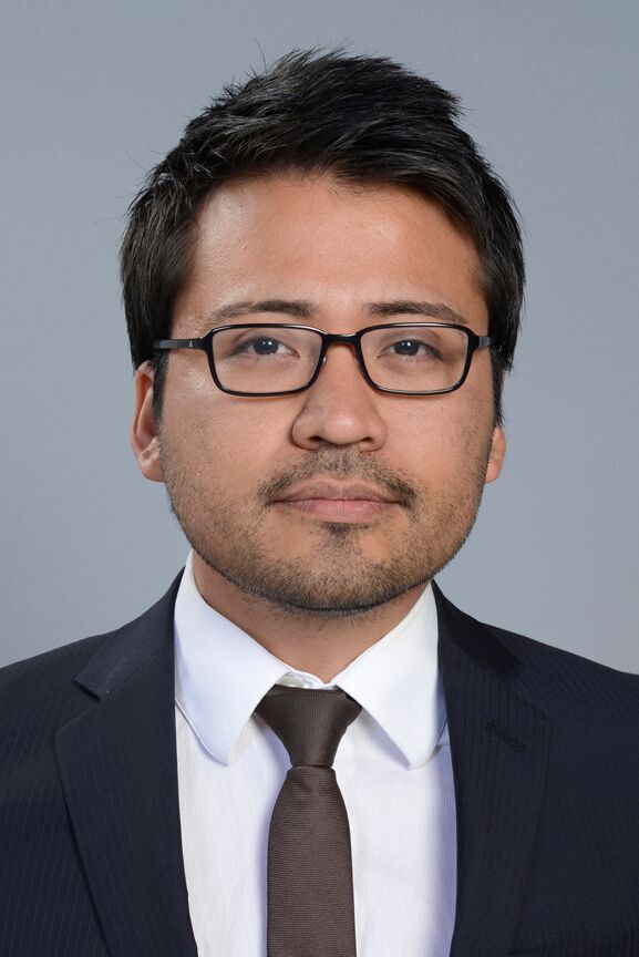
Carlos Aguirre
Faculty
Hello, I am Carlos. My research interests are: Applications of Machine Learning to Chemistry, Computational Chemistry, Chemical Simulations and Reactive Force Fields. My training is in Physics, Optics and Quantum Chemistry.
Yu-Ying Tzeng
Postdoctoral Fellow
Hello, I am Ying. My research interests are: Machine Learning, Deep Learning application, Monte Carlo methods, Risk Management and Insurance. My training is in Financial Mathematics.
Guanglei Xu
Postdoctoral Fellow
Hello, I am Guanglei Xu. My research interests are Quantum Algorithm development, Quantum Computing device design and application of Near-Term Quantum Computers and Quantum Simulators. My training is in Quantum Optics and Computation.
Gabriel Jurado
Graduate Student
Hello, I am Gabriel. My research interests are: Phase-Transitions, Critical Phenomena, Renormalization Group, Information Geometry, and Non-Equilibrium Dynamics. My training is in Theoretical Condensed Matter Physics.
Peter Woerner
Graduate Student
Hello, I am Peter. My research interests are: Engineering, Optimization, Hardware, Modeling and Simulation. My training is in Mechanical Engineering and Material Science.
Nathan Crock
Graduate Student
Hello, I am Nathan. My research interests are Representation Learning, Transfer Learning, and Learning without Backpropagation. My training is in Mathematics, Computational Science and Neuroscience.
Sara Victoria
Editor
Hello, I am Sara. My research interests are Foreign Languages and Linguistics. My training is in East Asian Languages/Culture and Psychology.
Alex Aduenko
Guest
Hello, I am Alex. My research interests are Financial Mathematics. My training is in Physics.
Miguel Agel Magaña Fuentes
Hello, I am Miguel. My training is in Computational Chemistry.
Henry Chung
Graduate Student
Hello, I am Henry. My research interests are Software Engineering, Website Development, and Weightlifting.
 "\tiny x\rightarrow \sigma(W\cdot x+b)")
&space;=&space;\frac{P(T_{train},&space;\theta|X_{train})}{\int&space;P(T_{train},&space;\theta|X_{train})\;\mathrm{d}\theta} "\tiny P(\theta|X_{train}, T_{train}) = \frac{P(T_{train}, \theta|X_{train})}{\int P(T_{train}, \theta|X_{train})\;\mathrm{d}\theta}")